Magnitude of eastward winds in the upper troposphere in the “fruit fly” model using the Earth’s rotation rate (bottom) and using a rotation rate that is 4 times larger (top). The red saturates at 50m/s eastward flow in the lower panel and 30 m/s in the upper panel. (Lat-lon plot over the entire globe — 50 Earth days of simulation in each clip.)
In post 28, I described a model of an ideal gas atmosphere with no latent heat (no water vapor for that matter) with radiative heating/cooling a function of temperature only, with no seasonal cycle, and with linear drag near the surface relaxing the flow back to zero in a rotating reference frame (this is how the atmosphere knows that it is rotating). The lower boundary condition is a homogeneous spherical surface (no mountains, no continents, no oceans). I think of this model as part of a hierarchy of models of increasing complexity so with an admiring reference to the way in which biological research is organizing around “model” organisms I refer to this as the “fruit fly” model. In that post, I mentioned that the surface westerlies move polewards as the rotation rate is decreased. Poleward movement of the westerlies is what we expect in a warming world. There is no guarantee that what we learn by varying the rotation rate in this very controlled setting will be directly relevant to that problem but I think it does stress our understanding in interesting ways . The animation above compares the evolution of the zonal (east-west) component of the wind in the upper troposphere when using the Earth’s rotation rate with the evolution you get with 4 times the Earth’s rotation rate.
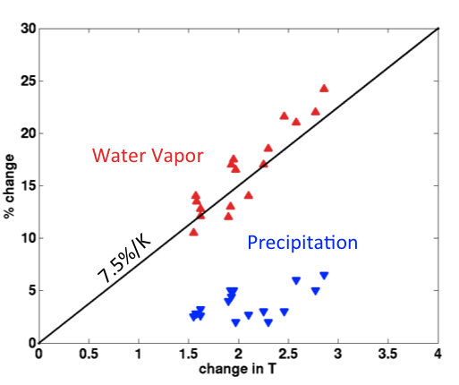
Fractional change in global mean precipitation (blue) and global mean (horizontally and vertically integrated) water vapor (red) as a function of change in global mean surface air temperature, over the 21st century in the A1B scenario in CMIP3 models. Redrawn from fig. 2 in Held and Soden 2006.
The figure at the top describes a very robust result in the responses to warming in global climate models: the fractional increase in the total amount of water vapor in the atmosphere is much larger than the fractional increase in global mean precipitation. While this figure shows the responses in CMIP3 models for a particular scenario of increasing forcing over the 21st century, the results from CMIP5 and different scenarios are all similar. This disparity in the magnitude of the increases in water vapor and precipitation and its important consequences for many other aspects of the climate response have been discussed since relatively early days in GCM simulations of climate change (e.g., Mitchell et al 1987). Perhaps the most fundamental consequence is the reduction in the vertical mass exchange between the lower and upper troposphere. That is, the “amount of convection” in the atmosphere decreases — or, by this particular measure, the atmospheric circulation slows down, especially in the tropics where a large fraction of this exchange takes place.
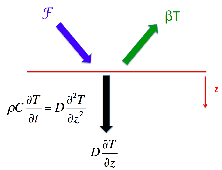
Vertical diffusion of heat has often been used as a starting point for thinking about ocean heat uptake associated with forced climate change. I have chosen instead to use simple box models for this purpose in these posts because they are easier to manipulate but also because I don’t feel that the simplest diffusive models bring you much closer to the underlying ocean dynamics. But diffusion does provide a simple way of capturing the qualitative idea that deeper layers of the ocean, and larger heat capacities, become involved more or less continuously as the time scales increase. So let’s take a look at the simplest possible diffusive model for the global mean temperature response. This model is typically embellished with a surface box, representing the ocean mixed layer, as well as by some attempt at capturing advective rather than diffusive transport (ie Hoffert, et al 1980, and Wigley and Schlesinger 1985), but let’s not worry about that. I want to use this model to make a simple point about the value of the concept of the transient climate response (TCR).
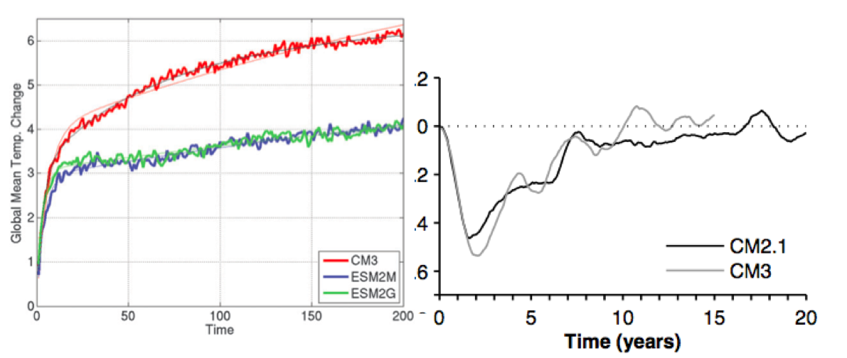
Left: The response to instantaneous quadrupling of CO2 in three GFDL models, from Winton et al, 2013a. Right: The ensemble mean response of global mean surface air temperature to Pinatubo in two GFDL climate models, from Merlis et al 2014.
This is a continuation of post #49 on constraining the transient climate response (TCR) using the cooling resulting from a volcanic eruption, specifically Pinatubo. In order to make this connection, you need some kind of model that relates the volcanic response to the longer time scale response to an increase in CO2. Our global climate models provide the logical framework for studying this connection. Using simple energy balance or linear response models to emulate the GCM behavior helps us understand what the models are saying. The previous post focused on one particular model, GFDL’s CM2.1. The figure on the right (from Merlis et al 2014 once again) compares the response to Pinatubo in CM2.1 with that in CM3, another of our models. The CM2 curve is an average over an ensemble of 20 realizations with different initial conditions; the CM3 curve is an average over 10 realizations. These two models have essentially the same ocean components but their atmospheric components differ in numerous ways. Most importantly for the present discussion, the different treatments of sub-grid moist convection result in CM3 being a more sensitive model to CO2 increase, whether measured by the TCR or the equilibrium response. One sees this difference in sensitivity in the left panel, showing the response to instantaneous quadrupling in three models, one of which is CM3. One of the others, ESM2M, is very closely similar to CM2.1 (it also has the option of simulating an interactive carbon cycle, driven by emissions rather than specified concentrations of CO2, so is referred to as an Earth System Model.) ESM2G has the identical atmospheric component as ESM2M but a different ocean model. As discussed in Winton et al 2013a, the different ocean models have little effect on this particular metric. The analogous simulation with CM2.1 would be very close to the green and blue curves in the left panel. Evidently the temperature responses to Pinatubo are not providing any clear indication that CM3 is the more sensitive model.
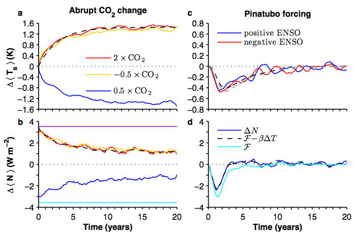
Some results on the response of a GCM (GFDL’s CM2.1) to instantaneous doubling or halving of CO2 (left) and to an estimate of the stratospheric aerosols from the Pinatubo eruption. From Merlis et al 2014.
The following is based on the recent paper by Merlis et al 2014 on inferring the Transient Climate Response (TCR) from the cooling due to the aerosols from a volcanic eruption. The TCR is the warming in global mean surface temperature in a model at the time of doubling of CO2 when the CO2 is increasing at 1% per year. You can generally convert the TCR of a model into a good estimate of the model’s warming due to the CO2 increase from the mid-19th century to the present, or due to all of the well-mixed greenhouse gases, by normalizing the TCR by the appropriate radiative forcing. The TCR of GFDL’s CM2.1 model, one of the two models discussed in Merlis et al, is 1.5K. Can you retrieve this value by looking at the model’s response to Pinatubo? This paper was motivated by the feeling that the literature trying to connect volcanic responses to climate sensitivity has focused too much on equilibrium sensitivity rather than directly constraining the TCR.
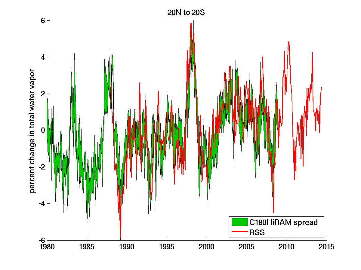
Percentage changes in total water vapor, vertically integrated and averaged over 20S-20N over the oceans only, comparing the RSS microwave satellite product (red) to the output of an atmospheric model running over prescribed SSTs (HADISST).
This is a continuation of the discussion in the previous post regarding the increase in water vapor near the surface and within the boundary layer more generally as the ocean surface warms. Models very robustly maintain more or less constant relative humidity in these lower tropospheric layers over the oceans as they warm, basically due to the constraint imposed by the energy balance of the troposphere on the strength of the hydrological cycle, and the tight coupling between the latter and the low level relative humidity over the oceans. Do we have observational evidence for this behavior? The answer is a definitive yes, as indicated by the plot above of microwave measurements of total column water vapor compared to model simulations of the same quantity. These are monthly means of water vapor integrated in the vertical. The observations are RSS Total Precipitable Water Product V7. The model is the 50km resolution version of GFDL’s HiRAM discussed in previous posts (on hurricane simulations , MSU trends , and land surface temperature trends) which uses observed SSTs and sea ice extent from HADISST1. for the lower boundary condition. Data are monthly means, deseasonalized by removing each month’s climatology defined by averaging over 1988-2007, and plotted as percentage changes from the climatological average over the same domain. The model results plotted are the spread of three realizations with different initial conditions (these are the runs from this model deposited in the CMIP5 database).
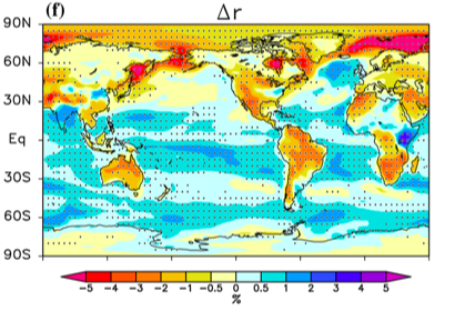
The change in near surface relative humidity averaged over CMIP5 models over the 21st century in the RCP4.5 scenario. Dec-Jan-Feb is on the left and June-July-Aug on the right. From Laine et al, 2014.
We expect the amount of water vapor in the atmosphere to increase as the atmosphere warms. The physical constraints that lead us to expect this are particularly strong in the atmospheric boundary layer over the oceans. The relative humidity (RH — the ratio of the actual vapor pressure to the saturation value) at the standard height of 2 meters is roughly 0.80 over the oceans. At typical temperatures near the surface, the fractional increase in the saturation vapor pressure per degree C warming is about 7%. So RH would decrease by about the same fraction, amounting to roughly 0.06 per degree C of warming if the water vapor near the surface did not increase at all. Why isn’t it possible for RH to decrease by this seemingly modest amount?
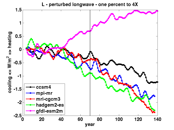
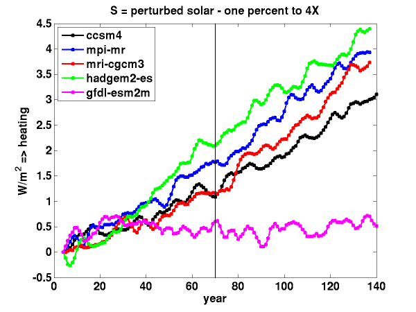
Evolution in time of fluxes at the top of the atmosphere (TOA) in several GCMs running the standard scenario in which CO2 is increased at the rate of 1%/yr until the concentration has quadrupled.
A classic way of comparing one climate model to another is to first generate a stable control climate with fixed CO2 and then perturb this control by increasing CO2 at the rate of 1%/yr. It takes 70 years to double and 140 years to quadruple the concentration. I am focusing here on how the global mean longwave flux at the TOA changes in time.
For this figure I’ve picked off a few model simulations from the CMIP5 archive (just one realization per model), computed annual means and then used a 7 yr triangular smoother to knock down ENSO noise, and plotted the global mean short and long wave TOA fluxes as perturbations from the start of this smoothed series. The longwave () and shortwave () perturbations are both considered positive when directed into the system, so is the net heating. The only external forcing agent that is changing here is CO2, which (in isolation from the effects of the changing climate on the radiative fluxes) acts to heat the system by decreasing the outgoing longwave radiation (increasing ). But in most of these models, L is actually decreasing over time, cooling the atmosphere-ocean system. It is an increase in the net incoming shortwave () that appears to be heating the system — in all but one case. This qualitative result is common in GCMs. I have encountered several confusing discussions of this behavior recently, motivating this post. Also, the ESM2M model that is an outlier here is very closely related to the CM2.1 model that I have looked at quite a bit, so I am interested in its outlier status.
Observed (HADCRUT4) surface temperature trends from 1980-2010, compared to the estimate of the forced response over this time frame obtained from the multi-model mean of the CMIP5 models. From Knutson et al 2013.
In the late 80’s, Mark Cane, Steve Zebiak and colleagues wrote a series of papers – Zebiak and Cane 1987 is one of the first – about a simple oscillatory atmosphere-ocean model of the tropical Pacific, with the goal of capturing the essence of ENSO evolution and providing dynamical predictions of ENSO. In 1996 Clement et al subjected this model’s surface temperatures to a forced warming tendency and showed that it then evolves towards a state that favors La Nina, and a cold Eastern Pacific, over the warm El Nino state.
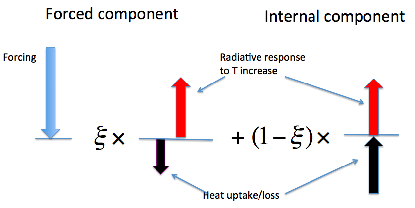
I’m returning to an argument discussed in post #16 regarding the decomposition of the global mean warming into a part that is forced and a part that is due to internal variability. I am not looking here for the optimal way of doing this decomposition. I am just interested in getting a better feeling for whether an increasing ocean heat content over time is a “smoking gun” for the forced component being dominant, a term Jim Hansen and others have used in this context. I’ll assume that we know that the heat flux has been into, not out of, the earth system (ie the oceans) averaged over the period in question, which could be the last half century or any period longer than a decade or two to insure that we can think in terms of a transient climate sensitivity (or transient climate response TCR) for the forced component. (AR5 WG1 Ch. 3 has a synthesis of the observations of ocean heat content). We’ll think in the most traditional terms, focusing on the global mean energy balance at the top of the atmosphere (TOA). Everything is considered to be a small perturbation from a control climate, and the assumption is that we can just linearly superpose the forced component of this perturbation and the component due to internal variability.


 ) and shortwave (
 ) perturbations are both considered positive when directed into the system, so
  is the net heating. The only external forcing agent that is changing here is CO2, which (in isolation from the effects of the changing climate on the radiative fluxes) acts to heat the system by decreasing the outgoing longwave radiation (increasing
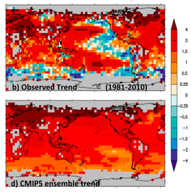
Recent Comments