18. Noise, TOA fluxes and climate sensitivity

Posted on October 7th, 2011 in Isaac Held's Blog

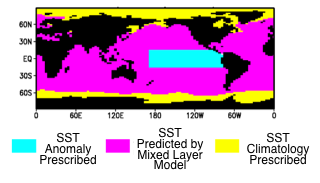A model configuration used to study how temperature variations in the equatorial Pacific force temperature variations in other ocean basins and the land. Figure courtesy of Gabriel Lau.

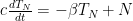
Consider a simple energy balance model for the oceanic mixed layer (+ land + atmosphere) with temperature $T$ and effective heat capacity $c$ . The net downward energy flux at the top-of-atmosphere $R$ is assumed to consist of a radiative relaxation, $- \beta T$ , plus some noise, $N$ . With imposed flux from the deep ocean to the mixed layer, $S$ :

$c \frac{dT}{dt} = R + S = -\beta T + N + S$

The assumption is that there is no external radiative forcing due to volcanoes or increasing CO2, etc. Can we use a simple one-box model like this to connect observations of interannual variability in $R$ and $T$ to climate sensitivity?

[This model is central to two papers by Spencer and Braswell (SB08, SB11). I provided a (signed) review for Journal of Climate of SB08, a fact that Spencer has publicized. My advice to simplify down to this one-box model, since it captures the essence of their argument, was followed by the authors. I was unclear on how best to estimate the ratio of the variances of $N$ and $S$ in this model — or, for that matter, whether this model was the appropriate setting for fitting to the data in question — so I didn’t address these issues in the review and recommended publication to let others work this out. I mention this since several people have asked me about my role in this paper.]

This is a linear equation that one can break up into the sum of two terms $T \equiv T_N + T_S$ , where

$c \frac{dT_N}{dt} = -\beta T_N + N$ , and $c \frac{dT_S}{dt} = -\beta T_S + S$ .

The key assumption is that $S$ and $N$ , and, therefore, $T_S$ and $T_N$ are uncorrelated — or $T_S$ and $N$ for that matter. Since we are interested in estimating $\beta$ from observations of $R$ and $T$ — a starting point might be regressing $R$ against $T$ , as in Forster and Gregory (2006). Defining

$\beta^* \equiv -[RT]/[T^2]$ .

where brackets are a time average, the difference between $\beta^*$ and $\beta$ is what we are interested in:

$\beta^* = \beta - [TN] /[T^2] = \beta - [T_N N] /[T^2]=\beta (1-[T_N^2]/[T^2])= \beta [T_S^2]/[T^2]$ .

The equation for $T_N$ has been used in setting $[T_N N]$ equal to $\beta [T_N^2]$ . One could stop here, or rewrite the last expression as

$\beta^* = \beta [S^2]/[S^2+N^2]$ .

(used by Murphy and Forster (2010)– MF10— in their critique of SB08), but there is actually no need to refer to $S$ — and we don’t need an evolution equation for $T_S$ . SB11 use this same model, looking at observed phase lags between $R$ and $T$ to argue that noise-generated temperatures must be significant in the observations.

The equation for $\beta^*$ holds if we filter all fields to emphasize certain frequency bands, so if one has some idea of the relative spectra of $T_N$ and $T_S$ , one could design the filter to reduce the effects of $T_N$ .

The meaning of $N$ and assumptions about its spectrum are the source of much of the confusion about this model, I think — at least it has been the source of my own confusion. In the simple model, $N$ is the variability that you have at the TOA if $T$ is fixed. You can try to estimate this fixed-T flux variance with a GCM. I looked at a few simulations with GFDL’s AM2.1 atmospheric model with fixed SSTs when I first saw the draft of SB08. They use 1.3 W/m² for the standard deviation of monthly means of $N$ , for a domain covering tropical oceans only, while AM2.1 with fixed SSTs produces 1.0 W/m² for the net radiation over the same domain, which did not raise any flags for me. (The model’s global mean noise amplitude in monthly means is abut 0.6 W/m².) In the GCM, this noise is essentially uncorrelated from month to month. In preparation for this post, I tried varying the parameters in the simple model over ranges that I thought were plausible, assuming that the decorrelation time for $N$ is no longer than a month, and could not generate cases with large enough $T_N$ to create significant ( > 10%) differences between $\beta^*$ and $\beta$ and phase lags in the right ballpark — if I push the parameters to create more noise in the temperatures (by reducing the heat capacity (depth) of the mixed layer, in particular) the TOA fluxes are too noisy. Returning to SB11, I noticed something that I missed the first time through, that they pass their “noise” through a 9-month top-hat smoother. If I do this and tune the noise variance, then things look more reasonable. But can “noise” with this spectrum be independent of $T_S$ (ie ENSO)? I personally can’t imagine how a model with fixed SSTs can produce TOA flux variations with this long a decorrelation time.

I think a more plausible picture is something like the following. The central and eastern tropical Pacific SSTs warm due to heat redistribution from below and relatively quickly warm the entire tropical troposphere; this stabilized atmosphere reduces convective cloudiness over the tropical Indian and Atlantic Oceans, reducing the reflection of the incident shortwave in particular, producing warming of these remote oceans that takes several months to build; the global or tropical mean temperature has a component that follows this remote oceanic response. So temperatures have a component forced by TOA flux anomalies, but these anomalies would not exist without the Pacific source of variability. (This is a caricature of the tropical atmospheric bridge described more fully by Klein et al 1999 in particular). The kind of model that is used to study this sort of thing is an atmosphere/land model, with prescribed ocean temperatures in the tropical Pacific, but with the rest of the ocean consisting of a surface mixed layer, either a uniform 50m slab of water or something more elaborate with a predicted depth, that adjusts its temperature according to the simulated surface fluxes (e.g. Lau and Nath (1999, 2003),. See the figure at the top of this post. It would be interesting to compare the results from this kind of model to tropical mean or global mean TOA flux observations.

A simple change in the box model that might capture a bit of this would be to set $N= N_0 + \alpha T_S$ , where $N_0$ is real atmospheric noise with appropriately short decorrelation time, and $\alpha$ is a constant that relates the remote change in TOA flux to ENSO. (Ignoring the time it takes to set up this flux response may be an oversimplification.) I would also give $T_S$ the spectrum of typical ENSO indices. This model generates phase lags without noise ( $N_0$ ), but adding some noise might still be useful.

Changes in tropical circulation associated with ENSO warmings are quite different from the circulation responses we expect from increases in CO₂, and cloud feedbacks in particular are presumably sensitive to these circulation changes. From the perspective of a climate modeler, one thing that I would look for, as discussed in posts #12 and #15, is if this co-variability of TOA fluxes and surface temperatures provides a metric that distinguishes between GCMs with different climate sensitivities. Actually, rather than equilibrium or transient climate sensitivity, I would look instead directly at the strength of the radiative restoring in transient warming runs — the canonical 1%/year CO2 growth simulations being the simplest. (The strength of radiative restoring changes in models as the system equilibrates (post #5), and equilibrium sensitivities are typically estimated by extrapolation in any case — while the transient climate response depends on ocean heat uptake processes that play little or no role in interannual variability). If GCM simulations of this co-variability are not somehow correlated across an ensemble of models with the radiative restoring that occurs when CO₂ increases, one would have to understand this, since it would suggests that the connection is not very direct. I am not aware of a paper that describes this correlation either in the CMIP3 or perturbed physics model ensembles in a comprehensive way — but I’m not aware of a lot of things.

[The views expressed on this blog are in no sense official positions of the Geophysical Fluid Dynamics Laboratory, the National Oceanic and Atmospheric Administration, or the Department of Commerce.]

9 thoughts on “18. Noise, TOA fluxes and climate sensitivity”

Science of Doom says:

October 8, 2011 at 5:24 am

I am glad to see this article.

I have been trying to understand the ocean depth value in the Murphy & Forster 2010 criticism of Spencer & Braswell 2008. (This was one part of their criticism of SB2008).

Murphy & Forster point out that the effect of the radiative noise (on accurate determination of climate sensitivity) is dependent on the ocean depth (in the model).

A good point.

What is less clear is what ocean depth is appropriate. I see their point about the time of the model run affecting the “effective ocean depth” because heat moves from the mixed layer into the deeper ocean over time. But it seems like an assumption that needs proof to say that the mixed layer depth in the model can simply increase. They simply increase the mixed ocean depth for the time period in question and rerun the model.

Looking at Mixed layer depth over the global ocean: An examination of profile data and a profile-based climatology, de Boyer Montegut et al, JGR (2004) I calculate a mean “mixed layer depth” of approx 60m. I did this “by eye” for each month from their charts for each 30′ of latitude and area weighted then averaged. (No response to email from de Boyer Montegut for the actual results so I can calculate it correctly).

This slightly arbitrary mixed layer is then linked to the deeper ocean via empirically determined “k”, e.g. from Hansen et al 1985, and many related papers.

I can’t find a paper which attempts to determine the effect of radiative noise on empirically determined climate sensitivity where a more realistic ocean model is used.

So I am currently attempting to produce these models in Matlab. The first pass with only a basic mixed ocean layer in Measuring Climate Sensitivity – Part One.

Since then I have created models with monthly varying ocean depth by latitude to see what effect the radiative noise has with realistic – and unrealistic variations – of this parameter.

And now I am working on a model with varying “k” (effective eddy conductivity) from the actual “mixed layer depth” into the deeper ocean (rather than just increasing the depth of the mixed layer which has infinite conductivity). All to see how the measurement of climate sensitivity is corrupted by radiation noise as these parameters are adjusted..

There may be some obvious flaws in this approach, or perhaps others have already demonstrated that mixed layer depth plus “effective conductivity” leads to the apparently unproven Murphy & Forster 2010 claim.

I would be interested in your advice or comments on this approach.
1. Isaac Held says:
  
  October 8, 2011 at 11:31 am
  
  There is quite a bit of literature on simple stochastic models of local SST spectra (ie. Frankignoul and Reynolds, 1983) that might help you think about this kind of issue (but on small spatial scales the focus is on surface and not TOA fluxes.) You may also find it useful to look at the kinds of 1D ocean models that people use who try to model the effects of ENSO on remote oceans (ie., Alexander et al, 2002 and refs therein) — I really think this is the key physical process at play here, not atmospheric noise. I am not sure how much effort one should put in to refining a one-box model of the global, or tropical, means.
2. Alexander Harvey says:
  
  October 8, 2011 at 2:03 pm
  
  SoD,
  
  I think that there are issues due to global averaging that cannot be resolved. If we have a world where the effective well mixed depth varies from location to location and perhaps also the strength of the restoring factor dF/dT varies from place to place, energy balance equations based on global averages become troublesome.
  
  Noisy short term fluctuations in the average temperature do not necessarily imply a change in the average TOA noise forcing nor the average TOA balance. They may do but I cannot see that the necessarily do. The relationships that exist locally to not necessarily result in meaningful global relationships.
  
  Similarly the effective globally averaged effective mixed layer depth could have an apparent variation in time where non actually exists. The initial averaged temperature response is likely due to just those regions where the WML is most shallow, as time passes the response comes from additional regions where the layer is thicker and hence the time constant is longer, resulting in an apparent change in the globally averaged depth of the mixed layer.
  
  I think that this is not only a plausible effect but the apparent one. The globally averaged temperature spectra is not in my view compatible with a globally homogeneous well mixed layer of constant depth. The slope of the spectral response with increasing frequency is not steep enough, being closer to that of a purely diffusive global layer. That is not to say that the WML doesn’t exist but simply that it is not homogeneous and the effects of averaging mimic a layer where the effective depth varies with the period of the signal.
  
  In general, I think one can be easily deceived by mimickry wheb working with global averages. I can construct noise models that mimic the general form and spectral content of the globally averaged temperature record to a high degree of accuracy but I am not sure that the results are meaningful.
  
  Isaac,
  
  I also have concerns about the relationship between an internal noise source and non-radiatively forced changes in the surface temperature. I could not rule out short term changes in the surface temperature due to variation in vertical temperature profile. E.G. the mixing of a stratified column results in lowering the surface temperature without any change in the heat content. I struggle to see how fluxes between the deeper layers and the surface layers can be nimble enough to result in the observed amplitude of the temperature noise at the surface on timescales as short as one month. I have no issue with longer period variations such as ENSO,
  
  Alex
eduardo says:

October 11, 2011 at 10:28 am

‘Actually, rather than equilibrium or transient climate sensitivity, I would look instead directly at the strength of the radiative restoring in transient warming runs — the canonical 1%/year CO2 growth simulations being the simplest. (The strength of radiative restoring changes in models as the system equilibrates (post #5), and equilibrium sensitivities are typically estimated by extrapolation in any case — while the transient climate response depends on ocean heat uptake processes that play little or no role in interannual variability). If GCM simulations of this co-variability are not somehow correlated across an ensemble of models with the radiative restoring that occurs when CO2 increases…….. ‘

I am a bit confused by this paragraph. In those transient experiments the non-blackbody restoring flux would be relatively unconstrained due to the different heat penetration in each model. Could the analysis of the co-variability between T and R in control runs be more adequate ?
1. Isaac Held says:
  
  October 11, 2011 at 12:19 pm
  
  Sorry for being obscure. I would indeed look at the regressions in a control experiment for starters. But I would then compare this, across models, with the radiative restoring in a 1%/yr C02 run — ie, looking at the change in net radiation per unit warming after taking out the radiative forcing. It is the response to CO2 we are interested in after all. This differs between models. We are looking for observables (the covariability of net radiation and global or tropical mean T on interannual time scales being a candidate) that can distinguish between models with smaller or larger responses to CO2. If you can’t do this, what is the basis for the claim that the observations are constraining “climate sensitivity”?
Troy_CA says:

October 16, 2011 at 12:01 pm

Dr. Held,

Dr. Spencer seems to have calculated the regression coefficient (TOA Flux – Forcing) vs. T_surface for the last 50 years of the 20th century experiment for the CMIP3 model runs:

http://www.drroyspencer.com/2011/10/our-grl-response-to-dessler-takes-shape-and-the-evidence-keeps-mounting/

Assuming that the model responses shown have indeed had the forcing removed from the TOA flux, it would seem pretty clear from those results that – at least using the models — you can’t simply represent the climate sensitivity as the inverse of the coefficients (indeed, many of them are negative!) However, to your specific point, it would be interesting to see whether the ECS of the models still shows some correlation to those calculated coefficients…perhaps it would be worth talking with Spencer to see if he could group those results according to the specific models?

Also, Dessler 2010 concludes that there is no correlation between the short-term/instantaneous cloud feedback and that of the long-term cloud feedback in the models, which would also suggest that the observed TOA flux vs. T using the FG06 method would not necessarily distinguish between those of differing ECS (particularly since the cloud response is the most important difference in determining those sensitivities).

Finally, I’d also note that the fact that the atmospheric temperature changes lag the sea surface temperature changes by several months, and thus only looking at the TOA flux (particularly for OLR) in sync with surface temperature changes will miss the larger atmospheric response.
1. Isaac Held says:
  
  October 16, 2011 at 2:09 pm
  
  At face value there is an indication of differences between observations and many of the models with regard to this regression coefficient. As mentioned by Eduardo in a previous comment, it would be simpler to look at control simulations of the models to avoid any need to estimate forcing. The key will be to understand what this regression is measuring.
  
  The lag between tropospheric temperatures and an El Nino index was, I think, first discussed by Pan and Oort, 1983. But my understanding is that there is little phase lag between tropical mean SSTs and tropospheric temperatures — most of the lag is between Nino3 or other ENSO indices and the tropical mean SST (see Sobel at al 2002).
Troy_CA says:

October 17, 2011 at 3:38 pm

Thanks, that Sobel et al paper is quite interesting. I agree that the lag between (for example) Nino3.4 and SST is greater than that between SST and tropospheric temperatures, but there still appears to be a lag on the scale of greater than a month between mean SST and tropospheric temperatures (perhaps my wording of “several” was an overstatement, I should’ve specified between 1-3 months as I go over here: https://troyca.wordpress.com/2011/10/03/quick-update-on-lag-between-sst-and-amsu-600-mb-with-daily-data/. Your paper mentions that “They [the SST_p and mean SST] are nearly synchronous with the atmospheric temperature”, but figure 2 shows a higher correlation between mean SST at both 1 and 2 months lag than it does at 0 months…perhaps I am misunderstanding, or we agree that 1-2 months can be considered nearly synchronous? If it is the latter, it would seem that using the FG06 method for determining climate sensitivity would still lead to an underestimate, due to the timing offset between the max OLR response from the atmosphere and that of the max SST, right?

Also, one of Science Of Doom’s commenters pointed to an interesting post by Dr. Spencer, which has a particular figure that may be of interest:

http://www.drroyspencer.com/wp-content/uploads/IPCC-5-yr-regression-based-sensitivities-1950-1999-vs-FT06.gif

(It’s from this post:

There, he is comparing what one gets as the result of using the FG06 method on the 20th Century runs vs. the known climate sensitivity of those models as determined by Forster and Taylor 2006.

Re: “it would be simpler to look at control simulations of the models to avoid any need to estimate forcing.” I believe Dessler 2011 used the control runs (figure 2), and eye-balling at zero lag, it appears the average regression slope is around 0.5 (corresponding to a ECS of let’s say 7-8 C according to the FG06 method), which is quite higher than the known sensitivity of those models. Of course, whether there is ANY relationship between that regression slope and the ECS would require knowing which lines are associated with which models.
1. Isaac Held says:
  
  October 17, 2011 at 5:45 pm
  
  According to some old notes (which I haven’t rechecked) using annual means the regression of global mean upward TOA flux vs global mean surface air temperature in a 1,000 year control run of our CM2.1 model is about 1.7 (W/m2)/K — with 2.0 for outgoing longwave and -03 for reflected shortwave (a coherencephase analysis shows substantial phase lags in the shortwave-temperature relation at almost all frequencies, but none in the longwave using annual means, so the shortwave number presumably has little to say directly about radiative restoring strength.) I don’t have the estimates of the sampling error in 10 year samples in these notes. I’m not sure how this number fits in with some of the plots you refer to — so I think I’ll wait for things to settle down. I don’t particularly see the motivation for going down to monthly time scales, where the noise level is higher, if one is interested in making some contact with climate sensitivity, except on the general principle that one shouldn’t have to throw out the information content in high frequencies if the techniques are appropriate.

Comments are closed.

Share this:

9 thoughts on “18. Noise, TOA fluxes and climate sensitivity”