31. Relative humidity in GCMs

Posted on September 1st, 2012 in Isaac Held's Blog

Relative humidity evolution over one year in a 50km resolution atmospheric model
in the upper (250hPa) and lower (850hPa) troposphere.

In their 1-D radiative-convective paper of 1967,  Manabe and Wetherald examined the consequences for climate sensitivity of the assumption that the tropospheric relative humidity (RH) remains fixed as the climate is warmed by increasing CO₂.  In the first (albeit rather idealized) GCM simulation of the response of climate to an increase in CO₂, the same authors found, in 1975, that water vapor did increase throughout the model troposphere at roughly the rate needed to maintain fixed RH. The robustness of this result in the world’s climate models in the intervening decades has been impressive to those of us working with these models, given the differences in model resolution and the underlying algorithms, a robustness in sharp contrast to the diversity of cloud feedbacks in these same models.

The animation above shows the evolution of RH on the 250hPa pressure surface in the upper troposphere and on the 850hPa surface in the lower troposphere  in a GCM (this is the same ~50km resolution model as discussed in several previous posts).  The loop covers one year with each frame showing a daily mean.  (This makes the animation a bit jumpy — I don’t have the a higher time resolution version of this field readily available.)  The brightest white is 100% relative humidity and darkest black 0%. Values less than 10% in the upper panel are common, in subsidence regions within the tropics or in stratospheric intrusions at higher latitudes. Air parcel trajectories cut though these pressure surfaces in complex ways and are difficult to visualize, these parcel trajectories being the key to understanding the resulting relative humidities. These animations can be useful in discussions with those unfamiliar with GCMs, who might mistakenly think that RH is fixed by fiat in these models.  The result that RH distributions remain more or less unchanged in warmer climates is an emergent property of these models.  Is it possible to construct a GCM that keeps the amount of water vapor itself more or less unchanged as the climate warms, rather than roughly following the saturation vapor pressure?  It would be nice to have such a model, which we could then analyze to see if it  provides as convincing a simulation of other aspects of the atmospheric circulation as do our existing GCMs.  But  no one has constructed such a model to my knowledge.

GCMs do simulate modest changes in the distribution of RH in response to increasing CO2.  In fact, there is actually considerable similarity across models in the pattern of RH change that is simulated, primarily reflecting an upward stretching of the troposphere and poleward expansion of the subtropical dry zones.  Here’s a figure from  Sherwood et al 2010 showing the mean relative humidity response, per degree C global surface warming, in the CMIP3 models, using the idealized scenario of a 1%/year increase in CO₂ and comparing the climate at the time of doubling to the control:

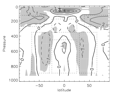Shading means that 16 of the 18 models being averaged over agree on the sign.  Averaging different models together reduces the amplitudes of the changes seen in individual models, but highlights the robust part of these changes.  You can look at the individual model results in the paper; individual models have larger amplitudes and more spatial structure in the pattern of the response,but they never approach the magnitude needed to compete with the temperature dependence of the saturation vapor pressure (more than 10%/C in the upper tropospheric regions of prime importance for water vapor feedback.)

Differences between the climatological RH in different models can be substantial,  and the biases in  these models compared to various observational estimates can be substantial as well (see, for example, the recent paper of Risi etal 2012 which also has quite a few references to other papers discussing these biases). Are these biases large enough to detract from our confidence in the robustness of the basic result that RH doesn’t change that much with warming? The situation is similar to that described in Post #26 on high-resolution simulations of radiative-convective equilibrium in small domains — different models simulate very different RH distributions associated with differences in the way that the convection is organized, but each model when warmed hold its RH distribution nearly fixed because the convective organization is effectively unchanged.

One can try to shed light on this robustness in global models by turning to the fruit fly model that I discussed in Post #28 — a dry ideal gas atmosphere on a sphere forced by relaxing temperatures to a specified “radiative equilibrium” field and relaxing near surface winds to zero.  Galewsky et al 2005 add a simple water-like passive tracer to this model — a tracer that does not interact with the flow or the temperatures.  It just has a specified source at the surface (“evaporation”) and a sink that exists only when the water vapor pressure rises above a saturation value that is a function of temperature, in which cases it just resets the vapor pressure to saturation, with the water vapor that disappears in this process thought of as “precipitation”.  The resulting time mean relative humidity is shown on the right.  The left panel is just the mean simulation from the AR4 models lifted form the Sherwood et al paper.

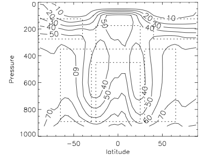
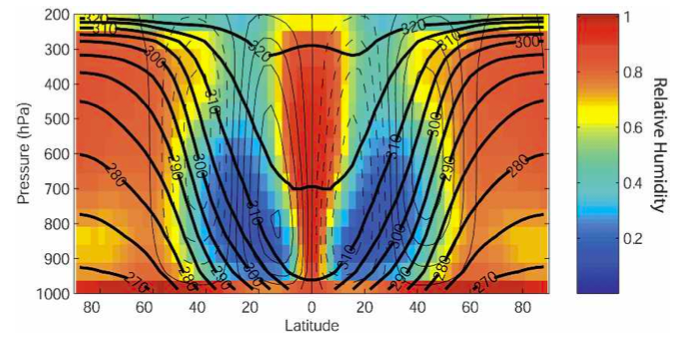
In the figure on the right, the bold lines are the mean potential temperature, or isentropic,  surfaces. Outside of the tropics, one can think of the air trajectories as tending to align along these surfaces.  Also shown with lighter lines (harder to see) are the streamlines of the mean meridional circulation — the time and zonally averaged circulation in the latitude-height plane, indicating mean upward motion at the equator and downward motion in the subtropics.

The most obvious feature that this model captures qualitatively is the subtropical dry zones. Air parcels in these driest areas have either been carried down and warmed due to compression by the mean subtropical subsidence after losing most of their water in upward motion near the equator — or they have traveled down the midlatitude isentropic surfaces after having condensed most of their water during an earlier poleward and upward excursion.  (The point of this paper was to think about how to quantify the relative importance of these two classes of trajectories.)  Differences with the comprehensive models on the left are due in part to the absence of realistic boundary layer mixing spreading the evaporated water upwards, the absence of  a seasonal cycle and monsoons that move subtropical dry zones and wash out the minima in the annual mean figure shown on the left, and the distortion of the vertical structure of the outflow from the tropical rising motion.  (In the dry model, this outflow is spread over a broad layer of the troposphere, whereas in more realistic models with moist convection this outflow is confined more sharply to a layer near 200mb, causing the dry zone to be displaced upwards compared to the passive water model.)  The bottom line is just that the atmospheric flow is what prevents this model atmosphere from becoming saturated everywhere – by wringing water out of parcels of rising/cooling air and then bringing these parcels back down so their relative humidity drops as they warm.

Suppose you warm this dry model.  There is an interesting special case that Tim Merlis and I have been discussing recently.  The relaxation to “radiative equilibrium” temperatures replaces radiative transfer in this model, so you  warm the model climate by warming these radiative equilibrium temperatures. Suppose also that the saturation vapor pressure is exactly exponential in temperature so that it increases by a fixed percentage for a uniform increase in temperature.  And then increase the evaporation by the same fraction.  One can show that the solution in this warmer climate will have exactly the same relative humidity as the original one — water vapor will increase everywhere by this same factor.  This is admittedly a very special situation —  it works only for the passive case,  so that the water vapor equation is linear, and is modified if the warming is non-uniform, but it provides a simple foundation for thinking about more complicated situations. (This is somewhat misleading — see the first comment and response below). I think more could be done with this passive-water fruit-fly model, helping us think about what kinds of changes in relative humidity can be generated by non-uniform warming and a changing mix of trajectories — without the added complexity of latent heat release and moist convection.

I’ll discuss some observed RH trends in upcoming posts.

[The views expressed on this blog are in no sense official positions of the Geophysical Fluid Dynamics Laboratory, the National Oceanic and Atmospheric Administration, or the Department of Commerce.]