

Posted on April 24th, 2014 in Isaac Held's Blog
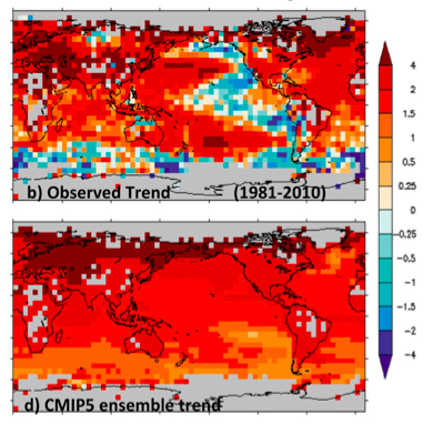 Observed (HADCRUT4) surface temperature trends from 1980-2010, compared to the estimate of the forced response over this time frame obtained from the multi-model mean of the CMIP5 models. From Knutson et al 2013.
In the late 80’s, Mark Cane, Steve Zebiak and colleagues wrote a series of papers – Zebiak and Cane 1987 is one of the first – about a simple oscillatory atmosphere-ocean model of the tropical Pacific, with the goal of capturing the essence of ENSO evolution and providing dynamical predictions of ENSO. In 1996 Clement et al subjected this model’s surface temperatures to a forced warming tendency and showed that it then evolves towards a state that favors La Nina, and a cold Eastern Pacific, over the warm El Nino state.
It is easy enough to understand why the Cane-Zebiak model tilts towards la Nina as it warms. On the ocean side, this is a model of the waters above the thermocline in the equatorial Pacific. Crucially, the temperature of the water upwelling into this layer from below is fixed as a boundary condition. Most of the upwelling occurs in the eastern Pacific. When the waters of the surface layer are warmed, the upwelling of water from deeper layers, assumed to be unaffected by the warming, retards the warming in the East but not the West, increasing the east-west temperature gradient across the Pacific. One can then envision the basic mechanism underlying ENSO kicking in to enhance the temperature gradient. Known as the Bjerknes feedback, a stronger east-west temperature gradient generates a precipitation distribution (more rain in the west, less in the east) that enhances the strength of the trade winds along the equator, pushing surface waters westward and enhancing the upwelling of cold waters in the east. The manner in which different negative feedbacks then develop due to slower transfers of heat between equatorial and off-equatorial waters is a main focus of ENSO theory, and these complicate matters, but presumably you can still think of la Nina conditions as being favored by upwelling waters that have not yet experienced warming.
The path taken by this water that upwells in the eastern Pacific is intricate. The major pathway is part of the shallow wind-driven overturning circulation. Subduction and last contact with the surface is primarily in the subtropics, mostly in the eastern half of the basin from where water masses can more easily drift westward and equatorward, typically reaching the western boundary first, where they proceed equatorward below the surface, eventually feeding the equatorial undercurrent which rises as it moves back eastward, mixing with surface waters in the east. An early paper describing the theory and modeling of this circulation is McCreary and Lu, 1994. See also the schematic in Fig. 3 of England et al, 2014. I was skeptical of the Clement et al result when it came out because of the extreme assumption that the upwelling waters are assumed not to have warmed at all. The time-scale of this shallow circulation is at most a decade or two, so one would have to visualize this modest delay being large enough to drive the system preferentially towards la Nina.
Waters subducted further polewards than the subtropics can also move equatorward and get caught up in the equatorial undercurrent and coastal (Peruvian) upwelling. Radiocarbon in tropical corals – Toggweiler et al 1991 – suggests that these denser source waters come from as far away as the Southern ocean north of the circumpolar current. This would lengthen the time lag, and maybe make it more plausible that the subsurface plumbing that emerges in our ocean models might be deficient.
Models don’t typically generate a la Nina like forced response, as seen in the figure at the top. The discrepancy does not just affect the usual hiatus period, the past 15 or so years, but as shown in the figure it affects trends over the full satellite era (causing the discrepancy between models’ and satellite (MSU) estimates of tropical tropospheric warming trends among other things). One possibility of course is that internal variability is the cause of this discrepancy between the observed and the forced component of the model trends. But the question here is whether the models could be missing a la Nina-like tendency in their forced responses.
In Held et al 2010, we tried to separate the response in our CM2.1 model, (in an ensemble of 20th century +A1B scenario simulations with stabilization of forcing agents after 2100) into fast and slow components with different spatial structures. We did this by returning all anthropogenic forcing agents to their pre-industrial values instantaneously at three times (2100, 2200, 2300). In response there is a fast cooling with e-folding time of just a few years, followed by a much slower “recalcitrant” cooling back to the pre-industrial climate. The slow part is computed by looking at what’s left 20 years following the instantaneous return to pre-industrial forcing, long enough for the fast part to have decayed away. The slow component can be thought of as the effect of the warming of the sub-surface waters on surface temperatures. The upshot is that the temperature response at any time is decomposed into two components, 


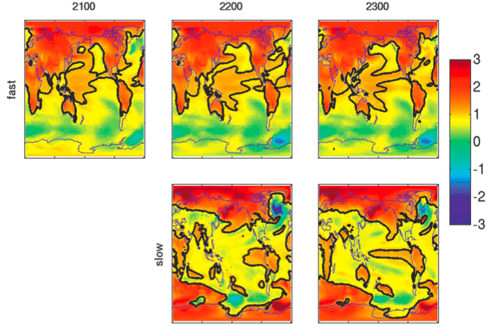 The fast part resembles la Nina, with larger warming in the western than in the eastern tropical Pacific. The slow part provides a complimentary El-Nino like pattern, more or less as one would expect from the dynamic retardation argument of Clement et al (I am avoiding the word “thermostat” because this mechanism is not maintaining a particular temperature.) You also get the sense of the different tropical responses imprinting themselves on the North Pacific as expected from the known responses to ENSO. I am not sure why this distinction between the equatorial Pacific structure of the fast and slow responses shows up clearly here and not so clearly within the 20th century part of these simulations, which should be dominated by the fast response. (The oversimplification of there being only two effective time scales is probably to blame — ie, some of the equatorial response in the slow component may not be as slow as the global mean recalcitrant component discussed in post #8.) I am pretty confused about the whole range of issues related to forced responses and free multi-decadal variability in the tropical Pacific. But maybe there is something to the simple idea that when warming starts kicking in rapidly enough, the eastern equatorial Pacific holds it back temporarily.
[The views expressed on this blog are in no sense official positions of the Geophysical Fluid Dynamics Laboratory, the National Oceanic and Atmospheric Administration, or the Department of Commerce.]
As our CO2 levels are now approaching mid-Pliocene levels, you might be interested to note this previous study that indicated that a La Nina (cool eastern Pacific) condition might have prevailed during this overall warmer period:
http://science.sciencemag.org/content/307/5717/1948
As rightly noted, this effect of “cooling” over the shorter period is temporary, as the overall lower sensible and latent heat flux brought about by this cool Eastern Pacific mode does not remove the energy from the climate system. Areas of valid research would be: Does this increase monsoon behavior and even more cyclone activity in the western Pacific? What does in mean for energy content in the IPWP (which research indicates was much greater during the mid-Pliocene). What about increased advection of energy toward the polar regions via ocean currents, that also seems to be indicated during the mid-Pliocene? Does the cool Eastern Pacific simply mean that energy will find another route to other parts of the climate system?
As I think you understand, the argument here has no particular relevance on time scales longer than the equilibration time of the part of the oceans that influence the near-surface waters of the equatorial Pacific.
Estimates of the state of the equatorial Pacific during the Pliocene have themselves fluctuated quite a bit — see Fedorov et al 2013 and Zhang et al 2014.
I think the Zhang paper provides compelling evidence against the old “Permanent El Nino” notion, which never made sense to begin with. I still think the paleo-community suffers from thinking about “El Nino” and “El Nino-like” as being dynamically interchangeable.
I think it made “sense” in the 1990’s and early 2000’s when people where looking for ways to link the strong El Nino’s of the 80’s and 90’s to global warming. Maybe the La Nina argument makes “sense” now because we’ve experienced a few of them. We are a fickle species. (apologies for the cynicism)
Can anybody link these ideas to the preponderance of La Nina from 1950-1975 in this index?
https://www.esrl.noaa.gov/psd/enso/mei/
Chris:
evidence against the old “Permanent El Nino” notion, which never made sense to begin with. I still think the paleo-community suffers from thinking about “El Nino” and “El Nino-like” as being dynamically interchangeable.
I would be careful with such generalizations. I think that there has certainly been a faction within the paleo community that had a rather unsophisticated and arguably unphysical view of ENSO during the Pliocene, but we should not make the mistake of believing that they are representative of the community as a whole, or even those who originated/still advocate for El Padre.
In fact, I would argue that a great deal of the incorrect “permanent El Niño” meme promotion came from interdisciplinary or not-primarily-paleo-focused people, but rather people whose primary expertise came from modern climate trying to tie El Niño to the warmer Pliocene due to perceived connections between contemporary greenhouse warming and ENSO.
There were some good sessions at Fall AGU 2013 about this very issue.
For starters, Kessler’s paper “Is ENSO a cycle or series of events?” demonstrates the evolution of ENSO events is loosely related to Bjerknes feedback, but not determined by the feedback itself, otherwise the longest El Nino on record during the 90’s, or similar double dip prolonged La Nina events at other times, would not be possible, as the length of these events are not strictly governed by more or less heat at one end of the gradient as Bjerknes feedback implies. Is La Nina the recharger, and El Nino the discharger? Such a simplification is doubtful, given that El Nino warms the climate, and heat generated via El Nino (thru water vapor, clouds, etc) eventually impacts the Western Pacific.
Add to this the unwavering stationarily of ENSO in a warming world (La Nina /El Nino is not getting stronger (statistically) as defined by SSTa), then the simplest explanation is that the “cycle or event” is independent of external forcing /warming.
The problem of going down the “independent road” so to speak, is that one is ignoring (or not understanding) why such an enormous climate phenomenon in terms of heat is so stable in the first place.
Sorry I’m a little confused by what the last graphs show. Especially because the paragraph before the graphs you are talking about cooling and after afterward about warming.
Putting aside the methodology, the point of this is to separate the warming in the model into 2 parts — one “fast” and one “slow”, “fast” and “slow” as compared to the time scale on which the main components of the forcing evolve. (The method of extracting the two parts involves taking a model that has already warmed and stripping away the forcing and watching it cool, but you don’t need to think about that when looking at the spatial structure of the two parts.) The amplitudes of two parts in this model is discussed in post #8 so I didn’t reproduce that here.