|
We begin by developing a terminology for describing the types of grids used in Earth System science models and datasets. Grids for Earth System science can be considerably specialized with respect to the more general grids used in computational fluid dynamics. Specifically, the vertical extent is considerably smaller (~10 km) than the horizontal (~1000 km), and the fluid in general strongly stratified in the vertical. The treatment of the vertical is thus generally separable; and model grids can generally be described separately in terms of a horizontal 2D grid with coordinates X and Y , and a vertical coordinate Z.
The underlying geometry being modeled is most often a thin spherical shell1, especially when it is the actual planetary dynamics that is being modeled. However, more idealized studies may use geometries that simplify the rotational properties of the fluid, such as an f-plane or β-plane, or even simply a cartesian geometry.
Where the actual Earth or planetary system is being modeled, geospatial mapping or geo-referencing is used to map model coordinates to standard spatial coordinates, usually geographic longitude and latitude. Vertical mapping to pre-defined levels (e.g height, depth or pressure) is also often employed as a standardization technique when comparing model outputs to each other, or to observations.
The vertical coordinate can be space-based (height or depth with respect to a reference surface) or mass-based (pressure, density, potential temperature). Hybrid coordinates with a mass-based element are considered to be mass-based.
The reference surface is a digital elevation map of the planetary surface. This can be a detailed topography or bathymetry digital elevation dataset, or a more idealized one such as the representation of a single simplified mountain or ridge, or none at all. Vertical coordinates requiring a reference surface are referred to as terrain-following. Both space-based (e.g Gal-Chen (missing ref: ), ζ (missing ref: )) and mass-based (e.g σ) terrain-following coordinates are commonly used.
The rationale for developing this minimal taxonomy to classify vertical coordinates is that translating one class of vertical coordinate into another is generally model- and problem-specific, and should not be attempted by standard regridding software.
Horizontal spatial coordinates may be polar (θ,φ) coordinates on the sphere, or planar (x,y), where the underlying geometry is cartesian, or based on one of several projections of a sphere onto a plane. Planar coordinates based on a spherical projection define a map factor allowing a translation of (x,y) to (θ,φ).
Curvilinear coordinates may be used in both the polar and planar instances, where the model refers to a pseudo-longitude and latitude, that is then mapped to geographic longitude and latitude by geo-referencing. Examples include the displaced-pole grid (Jones et al. 2005) and the tripolar grid (Murray 1996).
Horizontal coordinates may have the important properties of orthogonality (when the Y coordinate is normal to the X) and uniformity (when grid lines in either direction are uniformly spaced). Numerically generated grids may not be able to satisfy both constraints simultaneously.
A third type of horizontal coordinate often used in this domain is not spatial, but spectral. Spectral coordinates on the sphere represent the horizontal distribution of a variable in terms of its spherical harmonic coefficients. These coefficients can be uniquely mapped back and forth to polar coordinates based on Fourier and Legendre transforms, yielding uniformly spaced longitudes, and latitudes defined by a Gaussian quadrature. This grid specification will not consider spectral representations directly; rather, it assumes that the data have been transformed to polar coordinates, and only seeks to encode the truncation used to restrict the representation to a finite set of values.
Spectral coordinates on the plane have also recently been used in this domain. These methods generally employ spectral elements (Thomas and Loft 2002; Iskandarani et al. 2002) projecting the sphere onto a series of planes of finite spatial extent, within each of which the representation is spectral. Spectral elements are also uniquely bound to geospatial coordinates by a series of transforms, and it is in these coordinates that the data are assumed to have been written.
As for the fourth coordinate, time, it is already reasonably well-covered in the CF conventions. Both instantaneous and time-averaged values are represented. Key issues that still remain include the definition and treatment of non-standard calendars, and for simulation data, a standard vocabulary to define aspects of a running experiment, such as the absolute start time of the simulation.
In translating a data variable to a discrete representation, we must decide what aspects are necessary for inclusion in a standard grid specification. We have chosen two classes of operations that the grid standard must enable: vector calculus, differential and integral operations on scalar and vector fields; and conservative regridding, the transformation of a variable from one grid to another in a manner that preserves chosen moments of its distribution, such as area and volume integrals of 2D and 3D scalar fields. We recognize that higher-order methods that preserve variances or gradients may entail some loss of accuracy. In the case of vector fields, grid transformations that preserve streamlines are required.
To enable vector calculus and conservative regridding, the following aspects of a grid must be included in the specification:
A taxonomy of grids may now be defined. A discretization is logically rectangular if the coordinate space (x,y,z) is translated one-to-one to index space (i,j,k). Note that the coordinate space may continue to be physically curvilinear; yet, in index space, grid cells will be rectilinear boxes.
The most commonly used discretization in Earth system science is logically rectangular, and that will remain the principal object of study here. Beyond the simplest logically rectangular grids may include more specialized grids such as the tripolar grid of Murray (1996) shown in Figure 2 and the cubed-sphere grid of Rancic et al. (1996), shown in Figure 3.
|

|
Triangular discretizations are increasingly voguish in the field. A structured triangular discretization of an icosahedral projection is a popular new approach resulting in a geodesic grid (Majewski et al. 2002; Randall et al. 2002). An example of a structured triangular grid is shown in Figure 4 from Majewski et al. (2002). The grid is generated by recursive division of the 20 triangular faces of an icosahedron.

|
Numerically generated unstructured triangular discretization, such as shown in Figure 5 are often used, especially over complex terrain. High resolution models interacting with real topography increasingly use such unstructured grids. Section 3.4 visits the issue of the specification of such grids.
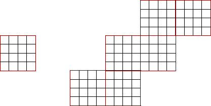
There is no need for unstructured grids to have only triangular elements (although we shall see in Section 2.6 that the supergrid abstraction allows us to build all such grids out of UTGs). Unstructured polygonal grids of arbitrary polygonal elements are a completely general abstraction, where each cell might have any number of vertices. In practice, we usually find somewhat more restrictive formulations such as in Spectral Element Ocean Model (SEOM) of Iskandarani et al. (2002) cited earlier: an example SEOM grid for the ocean is shown in Figure 6.
A reasonably complete taxonomy of grid discretizations for the near- to mid-future in Earth System science would include:
While developing a vocabulary and placeholders for all of the above, we shall focus here principally on logically rectangular discretizations. We shall expose the key concepts of supergrids (Section 2.6) and mosaics (Section 2.7) based on LRGs, and aim to show their relevance for other discretization types as well. We expect the specification to be extended to these other discretization types by the relevant domain experts, as in Section 3.4.
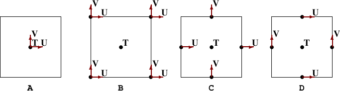
Algorithms place quantities at different locations within a grid cell (“staggering”). In particular, the Arakawa grids, covered in standard texts such as Haltiner and Williams (1980) show different ways to represent velocities and masses on grids, as shown in Figure 8.
This has led to considerable confusion in terminology and design: are the velocity and mass grids to be constructed independently, or as aspects (“subgrids”) of a single grid? How do we encode the relationships between the subgrids, which are necessarily fixed and algorithmically essential?
In this approach, we dispense with subgrids, and instead invert the specification: we define a supergrid. The supergrid is an object potentially of higher refinement than the grid that an algorithm will use; but every such grid needed by an application is a subset of the supergrid.
Given a complete specification of distances, angles, areas and volumes on a supergrid, any operation on any Arakawa grid is completely defined.
The refinement of an Arakawa grid is always 2: here we generalize the refinement factor to an arbitrary integer, so that a single high-resolution grid specification may be used to run simulations at different resolutions.
We can now define a cell without ambiguity: it is an element of a supergrid. A cell on the grid itself may be overspecified, but this guarantees that any set of staggered grids will have consistent coordinate distances and areas.
The supergrid cell itself does not have a “center”: in constructing a grid from a supergrid, the grid center is indeed a vertex on the supergrid. However, certain applications of supergrids require the specification of a centroid (e.g Jones 1999), a representative cell location. This is nominally some the center of some weighting field distributed about its area; but it is incorrect to try and compute a distance from centroid to a vertex.
Staggered arrays may be defined as symmetric or asymmetric arrays. Taking the
Arakawa C-grid (Figure 9) as an example, we have a 8×8 supergrid. Scalars,
at cell centres, will form a 4×4 array. A symmetric array representing the
velocity component U will be of size 5×4. Quite often, though, all arrays may be
defined to be 4×4, in which case, one must also specify if the U points are
biased to the “east” or “west”, i.e if the array value u(i,j) refers to the
point U(i +  ,j) or U(i -
 ,j). While this can be inferred from the array
size, it is probably wise to include this information in the specification for
readability.
,j). While this can be inferred from the array
size, it is probably wise to include this information in the specification for
readability.
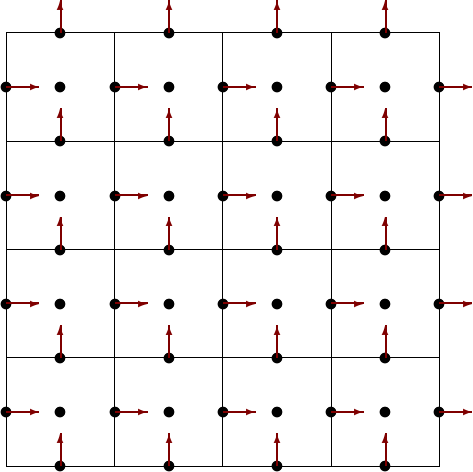
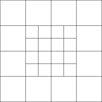
Grid refinement is another application of supergrids. A refined grid is usually a fine grid overlying a coarse grid, with some integer factor of resolution in index space. The vertices on the coarse grid are also vertices on the fine grid, as shown in the example of Figure 10.
|
The coincidence of certain vertices of refined grids in contact permit certain operations more specialized than the completely generalized overlap contact region specified in Section 2.9. The supergrid plays a role here, as the vertices of a single logically rectangular supergrid can capture all of the grid information for a refined grid. Of course, adaptive refinement techniques where grids may be indefinitely refined may not allow for the prior definition of that supergrid.
Can the supergrid idea be extended to non-rectangular grids? It is somewhat less intuitive in this case, but it is argued in this article that the supergrid idea is equally applicable to grids that are not logically rectangular. There are several reasons to attempt to encode unstructured grids in this fashion. First, we see in the STG of Figure 4 that coarse resolution grids, say at ni = 1, 2 or 4, can be constructed by subsampling a supergrid defined at ni = 8. Second, staggering is a concept equally at home on triangular grids. It is common practice on STGs and UTGs to define vertex-, cell-, and face-centered quantities. Furthermore, several key interpolative algorithms on UTGs depend on these quantities, as shown in Figure 11 from Majewski et al. (2002).
The proposed treatment of unstructured grids, detailed below in Section 3.4, is to define a specification of UTGs that represent a supergrid, i.e including all vertex-, cell-, and face-centered locations. Only UTGs need to be considered in defining a supergrid, as a triangular supergrid underlies any unstructured grid, including those containing polygons with arbitrary vertex counts.
Raster grids are a discretization of a surface into high-resolution pixels of an atomic nature: a “point” is the location of its containing raster, and any “line” is made up of discrete segments that follow raster edges but which cannot intersect them. The “area” of any grid cell on a raster is defined merely by counting the pixels within its bounding curve.
An application of raster grids is the use of catchment grids or PCGs (Koster et al. 2000). Catchment grids follow digital elevation isolines to form bounding boxes following topography to facilitate modeling land surface processes. PCGs are defined entirely in terms of an underlying raster grid.
A raster grid can also be defined on the basis of a high-resolution supergrid. Typically, these are created on the basis of high-resolution digital elevation datasets defined on a sphere. Thus raster grids are defined here as LRG supergrids. The centroid defines the raster location.
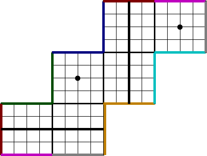
In many applications, it makes sense to divide up the model into a set of grid tiles2, each of which is independently discretized. An example above is the cubed-sphere of Figure 3, which is defined by six grid tiles, on which a data field may be represented by several arrays, one per tile. We call such a collection of grid tiles a grid mosaic, as shown in Figure 12.
|
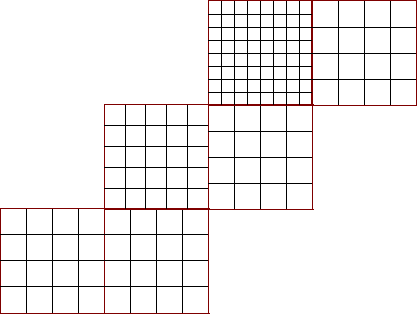
A grid mosaic is constructed recursively by referring to child mosaics, with the tree terminating in leaves defined by grid tiles (Figure 13).
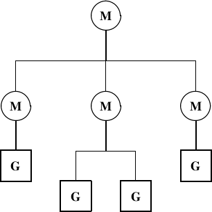
|
Aside from the grid information in the grid tiles, the grid mosaic additionally specifies connections between pairs of tiles in the form of contact regions between pairs of grid tiles.3
Contact regions can be boundaries, topologically of one dimension less than the grid tiles (i.e, planes between volumes, or lines between planes), or overlaps, topologically equal in dimension to the grid tile. In the cubed-sphere example the contact regions between grid tiles are 1D boundaries: other grids may contain tiles that overlap. In the example of the yin-yang grid (Kageyama et al. 2004) of Figure 14 the grid mosaic contains two grid tiles that are each lon-lat grids, with an overlap. The overlap is also specified in terms of a contact region between pairs of grid tiles. Issues relating to boundaries are described in Section 2.8. Overlaps are described in terms of an exchange grid (e.g Balaji et al. 2006a), outlined in Section 2.9.

|
The grid mosaic is a powerful abstraction making possible an entire panoply of applications. These include:
All of these applications make the grid mosaic abstraction central to this specification.
Boundaries for LRG tiles are specified in terms of an anchor point and an orientation. An anchor point is a boundary point that is common to the two grid tiles in contact. When possible, it is specified as integers giving index space locations of the anchor point on the two grid tiles. When there is no common grid point, the anchor point is specified in terms of floating point numbers giving a geographic location. The orientation of the boundary specifies the index space direction of the running boundary on each grid tile.
Figure 16 shows an example of boundaries for the cubed-sphere grid mosaic. Colored lines show shared boundaries between pairs of grid tiles: note how orientation may change so that a “north” edge on one grid tile may be in contact with a “west” edge of another. Orientation changes indicate how vector quantities are transformed when transiting a grid tile boundary.
Note that cyclic boundary conditions can be expressed as a contact region of a grid tile with itself, on opposite edges, and the polar fold in Figure 2 likewise.
Boundary conditions are considerably simplified when certain assumptions about grid lines can be made. These are illustrated in Figure 17 for various types of boundaries.
A boundary has the property of alignment when there is an anchor point in index space shared by the two grid tiles, i.e it is possible to state that some point (i1,j1) on grid tile 1 is the same physical point as (i2,j2) on grid tile 2. An aligned boundary has no refinement when the grid lines crossing the boundary are continuous, as in grid tiles 1 and 2 in Figure 17. The refinement is integer when grid lines from the coarse grid are continuous on the fine grid, but not vice versa, see grid tiles 5 and 6. The refinement is rational in the example of tile 3, when the contact grid tiles have grid line counts that are co-prime.
These properties, if present, will aid in the creation of simple and fast methods for transforming data between grid tiles. If none of the conditions above are met, there is no alignment. Anchor points are then represented by geo-referenced coordinates, and remapping is mediated by an exchange, as described below in Section 2.9.
When there are overlapping grid tiles, the exchange grid construct of Balaji et al. (2006a) is a useful encapsulation of all the information for conservative interpolation of scalar quantities.4 The exchange grid, defined here, does not imply or force any particular algorithm or conservation requirement; rather it enables conservative regridding of any order. Methods for creation of exchange grids are briefly discussed, but the standard is of course divorced from any implementation.
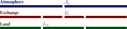
Given two grid tiles, an exchange grid is the set of cells defined by the union of all the vertices of the two parent grid tiles. This is illustrated in Figure 18 in 1D, with two parent grid tiles (“atmosphere” and “land”). (Figure 19 shows an example of a 2D exchange grid, most often used in practice). As seen here. each exchange grid cell can be uniquely associated with exactly one cell on each parent grid tile, and fractional areas with respect to the parent grid cells. Quantities being transferred from one parent grid tile to the other are first interpolated onto the exchange grid using one set of fractional areas; and then averaged onto the receiving grid using the other set of fractional areas. If a particular moment of the exchanged quantity is required to be conserved, consistent moment-conserving interpolation and averaging functions of the fractional area may be employed. This may require not only the cell-average of the quantity (zeroth-order moment) but also higher-order moments to be transferred across the exchange grid.
Given N cells of one parent grid tile, and M cells of the other, the exchange grid is, in
the limiting case in which every cell on one grid overlaps with every cell on the other,
a matrix of size N × M. In practice, however, very few cells overlap, and
the exchange grid matrix is extremely sparse. In code, we typically treat the
exchange grid cell array as a compact 1D array (thus shown in Figure 18 as
 rather than
  )
with indices pointing back to the parent grid tile cells. Table 1 shows the characteristics
of exchange grids at typical climate model resolutions. The first is the current GFDL
model CM2 (Delworth et al. 2006), and the second for a projected next-generation
model still under development. As seen here, the exchange grids are extremely
sparse.
)
with indices pointing back to the parent grid tile cells. Table 1 shows the characteristics
of exchange grids at typical climate model resolutions. The first is the current GFDL
model CM2 (Delworth et al. 2006), and the second for a projected next-generation
model still under development. As seen here, the exchange grids are extremely
sparse.
|
|
The computation of the exchange grid itself could be time consuming, for parent grid tiles on completely non-conformant curvilinear coordinates. In practice, this issue is often sidestepped by precomputing and storing the exchange grid. The issue must be revisited if either of the parent grid tiles is adaptive. Methods for exchange grid computation include the SCRIP package (Jones 1999) and others based on discretizing the underlying continuous geometry as a raster of high-resolution pixels (Koster et al. 2000).
This illustration of exchange grids restricts itself to 2-dimensional LRGs on the planetary surface. However, there is nothing in the exchange grid concept that prevents its use in any of the discretizations of Section 2.5, or in exchanges between grids varying in 3, or even 4 (including time) dimensions.
A complication arises when one of the surfaces is partitioned into complementary
components: in Earth system models, a typical example is that of an ocean and
land surface that together tile the area under the atmosphere. Conservative
exchange between three components may then be required: quantities like
CO have reservoirs in all three media, with the total carbon inventory being
conserved.
have reservoirs in all three media, with the total carbon inventory being
conserved.
|
|
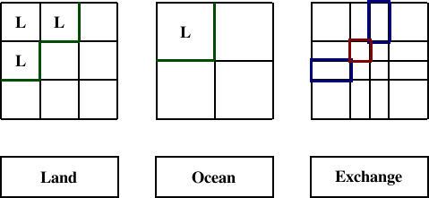
Figure 19 shows such an instance, with an atmosphere-land grid and an ocean grid of different resolution. The green line in the first two frames shows the land-sea mask as discretized on the two grids, with the cells marked L belonging to the land. Due to the differing resolution, certain exchange grid cells have ambiguous status: the two blue cells are claimed by both land and ocean, while the orphan red cell is claimed by neither.
This implies that the mask defining the boundary between complementary grids can only be accurately defined on the exchange grid: only there can it be guaranteed that the cell areas exactly tile the global domain. Cells of ambiguous status are resolved here, by adopting some ownership convention. For example, in the FMS exchange grid, we generally modify the land model as needed: the land grid cells are quite independent of each other and amenable to such transformations. We add cells to the land grid until there are no orphan “red” cells left on the exchange grid, then get rid of the “blue” cells by clipping the fractional areas on the land side.
1Except at very fine scales, the geometry is treated as a sphere, not a geoid. This may be a problem when geo-referencing to very precise datasets that consider the surface as a geoid.
2The words grid and tile separately are overused, and can mean many things depending on context. We will somewhat verbosely try always to use the term grid tile to avoid ambiguity.
3It is not necessarily possible to deduce contact regions by geospatial mapping: there can be applications where geographically collocated regions do not exchange data, and also where there is implicit contact between non-collocated regions.
4Streamline-preserving interpolation of vector quantities between grids is still under study, and may result in extensions to this proposed grid standard.