4.   Examples

4.1.   Cartesian geometry

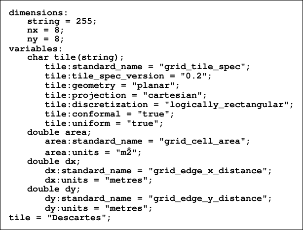(10)

The Cartesian grid spec of CodeBlock 10 illustrates several simplifications with respect to CodeBlock 3.

• The geometry:planar attribute (Section 2.1) indicates that geo-referencing is not possible.
• Since the uniform attribute (Section 2.3) is set, the area, dx and dy fields reduce to simple scalars.
• The combination of a conformal attribute and the planar geometry means that it is not required to store angles: grid lines are orthogonal, and that’s that.
• The tile name is of course arbitrary: we have chosen to type the tile as a string to avoid using the derived or complex types of netCDF-4. Mosaic processing tools will enforce the absence of two tiles bearing the same name.

Note that this gridspec might actually represent a supergrid of a 4×4 grid: we cannot tell from the gridspec alone. We would need to examine a field containing a physical variable (Section 3.6).

4.2.   Gaussian grid

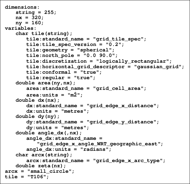(11)

(12)

A Gaussian grid is a spatial grid where locations on a sphere are generated by “Gaussian quadrature” from a given truncation of spherical harmonics in spectral space.

• There is no projection onto a plane.
• Since this is a regular grid (Section 2.3), dx and dy are 1D rather than 2D arrays. The specification of angles is similarly reduced by the conformal attribute.
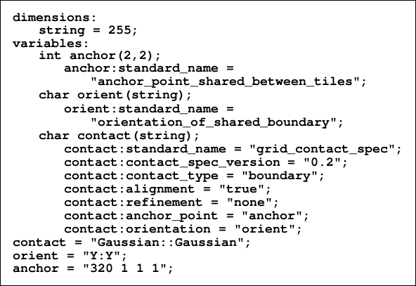
• The contact spec in CodeBlock 12 specifies periodicity in X.
• The associated mosaic specification is not shown here, as a simple Gaussian grid is a mosaic of a single tile. The horizontal_grid_descriptor (Section 3.2) is given a value of spectral_gaussian_grid: this value belongs to a controlled vocabulary of grid descriptors. The combination of this descriptor with the truncation level is enough to completely specify the gaussian grid.

4.3.   Reduced gaussian grid

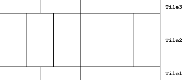
A Gaussian grid is of course a kind of regular_lat_lon_grid, and can suffer from various numerical problems owing to the convergence of longitudes near the poles. The reduced Gaussian grid of Hortal and Simmons (1991) overcomes this problem by reducing the number of longitudes within latitute bands approaching the pole, as shown in Figure 20.

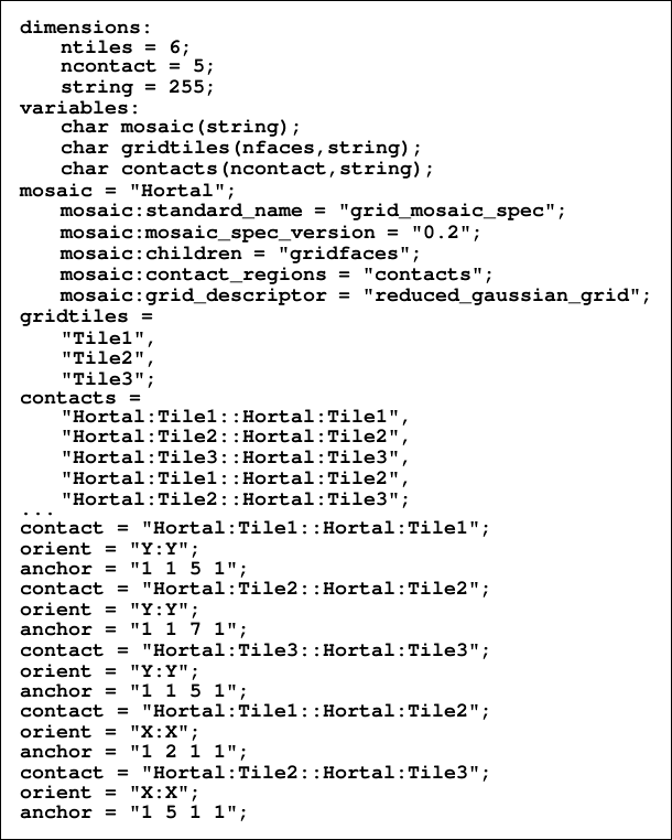(13)

The reduced Gaussian grid of Figure 20 is represented as a mosaic of multiple grid tiles, each of which is restricted to a latitude band, and has different longitudinal resolution.

• The mosaic as a whole has the reduced_gaussian_grid descriptor.
• It consists of 3 tiles, as shown in Figure 20, and 5 contact regions. The first 3 contacts express periodicity in X within a tile; the last two express contacts between tiles at the latitude where the zonal resolution changes.

4.4.   Tripolar grid

The tripolar grid of Figure 2 is a LRG mosaic consisting of a single tile. The tile is in contact with itself in the manner of a sheet of paper folded in half. In the X direction, we have simple periodicity. Along the north edge, there is a fold, which is best conceived of a boundary in contact with itself with reversed orientation. Thus, given a tripolar grid called murray of M × N points, we would have:

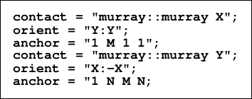(14)

4.5.   Unstructured triangular grid

We show here an example of fields on a UTG following the FVCOM example of Section 3.4. The example shows vertex-centred scalars and cell-centered velocities:

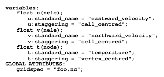(15)

balajiprinceton.edu