Arctic Sea Ice Predictions
Contacts, for more information:
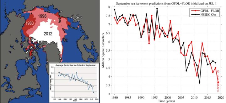
Continuous observations of the Arctic sea-ice cover have been possible since 1979 with the use of passive microwave satellite instruments. The minimum of Pan-Arctic sea-ice extent occurs each year in September. Since the beginning of the satellite record, September sea-ice extent has decreased by about 40%. Large year-to-year fluctuations are superimposed on this long-term decline, such as the 1996 maximum, and the 2007 and 2012 minima. Predicting these interannual fluctuations is critically important to improve management of ocean and coastal resources in the Arctic, better serve Northern communities, and provide planning information for shipping industries.
While the long-term sea-ice decline can be well reproduced by climate models forced by historical radiative forcing, the models need to be initialized from the observed climate state in order to capture year-to-year variations. GFDL has developed a quasi-operational prediction system that is run every month and produces seasonal forecasts of the climate system, including sea-ice extent. GFDL seasonal predictions are initialized every month from the Ensemble Kalman Filter Data Assimilation system built on the CM2.1 model (Zhang et al. 2007), which provides realistic ocean, sea ice, atmosphere and land initial conditions to the predictions. Seasonal predictions are run using the CM2.1 model as well as the Forecast-oriented Low Ocean Resolution (FLOR) model, which has the same ocean-sea ice resolution as CM2.1 but a finer atmospheric resolution. GFDL routinely submits sea ice forecasts to the September Sea Ice Outlook and to the Sea Ice Prediction Network.
Regional Arctic Sea Ice Prediction Skill
Retrospective seasonal predictions performed with CM2.1 and FLOR show skill in predicting detrended Pan-Arctic sea-ice extent anomalies at lead times of 1-6 months (Msadek et al. 2014). The prediction skill of CM2.1 and FLOR are similar, highlight the key importance of their common ocean and sea ice initial conditions (Msadek et al. 2014). While pan-Arctic sea ice extent predictions are a crucial first step, their utility is somewhat limited for stakeholders, who are primarily interested in sea ice predictions on regional and sub-regional spatial scales. Regional sea ice predictions are a pressing need for a broad stakeholder group, including northern communities, wildlife, shipping industries, fisheries, and natural resource industries. Motivated by this, GFDL has placed an emphasis on assessing sea ice predictions on stakeholder-relevant spatial scales. The FLOR and CM2.1 models have been shown to skillfully predict regional sea ice in both summer and winter (Bushuk et al. 2017a). The regional SIE prediction skill generally exceeds that of a persistence forecast, with notably high skill for winter sea ice extent in the North Atlantic sector. Summer regional predictions are skillful at 1-4 months in advance and display a barrier of prediction skill corresponding to initial month May. North Pacific regional sea ice predictions were found to have lower skill than their North Atlantic counterparts.
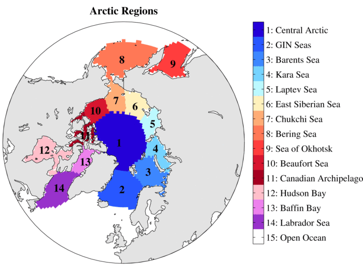 The Arctic regional domains considered in this skill assessment.
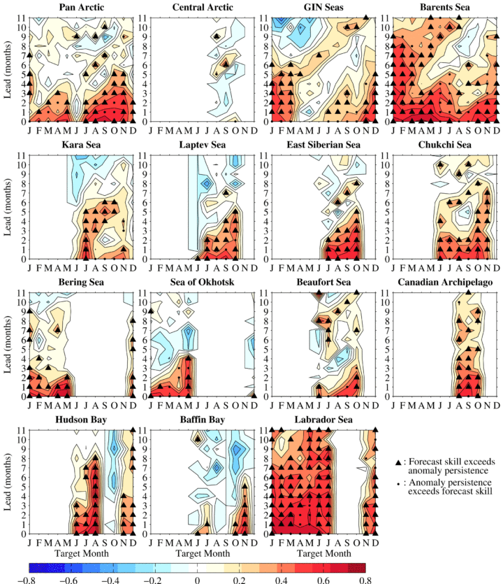 Seasonal prediction skill (ACC) for detrended regional Arctic SIE. The triangle and dot markers indicate months in which the ACC values are statistically significant at the 95% confidence level. Triangles indicate months in which the dynamical model’s skill exceeds that of a persistence forecast, and circles indicate months in which the persistence forecast exceeds the model’s skill.
Potential Predictability of Arctic Sea Ice
How much room for improvement do we have for regional sea ice predictions? A suite of perfect model predictability experiments was run with the FLOR model to explore this question. Bushuk et al. (2018) provided the first comparison between operational and perfect model skill using a common dynamical prediction system. In nearly all Arctic regions, they report a significant gap between perfect model and operational skill, indicating potential for improved regional predictions in future seasonal forecast systems. The skill structures are generally similar between the perfect model and operational predictions, including long-lead prediction skill for winter sea ice in the North Atlantic, lower skill in the North Pacific, and the presence of a spring predictability barrier for summer sea ice predictions. Further work exploring the predictability of CMIP5 models showed that this spring predictability barrier is a robust feature across CMIP5 models (Bonan et al. 2019). The spring barrier implies a relatively sharp limit on the potential skill of regional summer sea ice predictions, and emphasizes a need for high-quality observations in the months of May and June. Other work has identified a link between persistence and predictability in GCMs, showing that intermodel differences in predictability can largely be explained by differences in their sea ice persistence (Blanchard-Wrigglesworth and Bushuk, 2018).
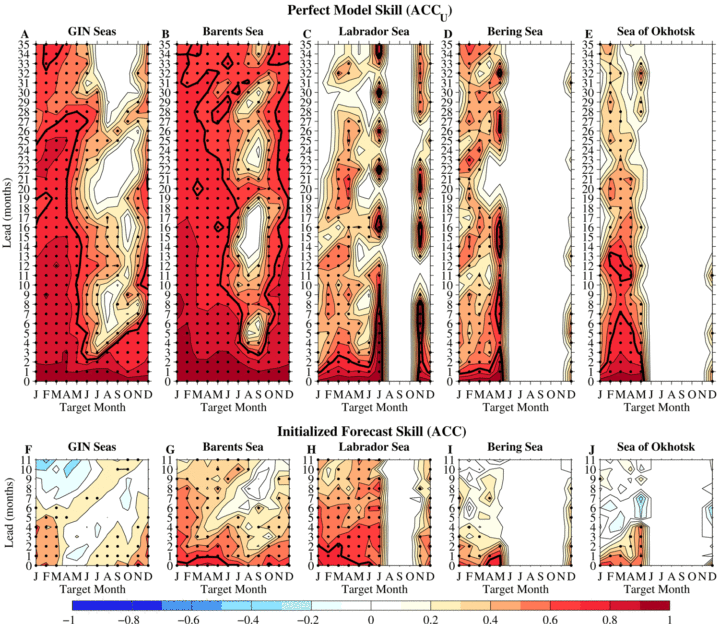 Comparison of perfect model (top row) and operational (bottom row) prediction skill for Arctic regional SIE for the GIN, Barents, Labrador, and Bering Seas and the Sea of Okhotsk. ACC values are plotted as a function of target month and forecast lead time. The thick black lines indicate the ACC=0.7 contours. Dots indicate months in which the ACC values are statistically significant at the 95% confidence level.
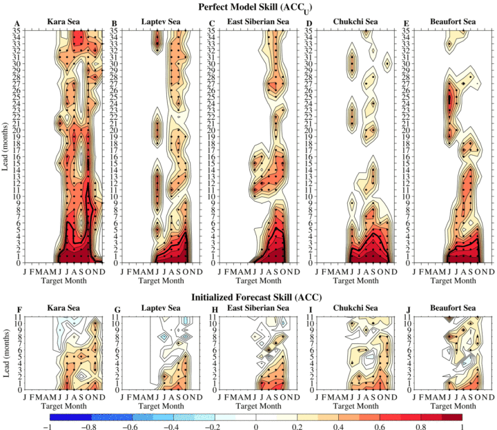 Comparison of perfect model (top row) and operational (bottom row) prediction skill for Arctic regional SIE for the Kara, Laptev, East Siberian, Chukchi, and Beaufort Seas. ACC values are plotted as a function of target month and forecast lead time. The thick black lines indicate the ACC=0.7 contours. Dots indicate months in which the ACC values are statistically significant at the 95% confidence level.
Mechanisms for Sea Ice Predictability
Why are GFDL sea ice predictions skillful? Ocean and sea ice initial conditions from ECDA have been shown to provide a crucial source of prediction skill for both winter and summer regional sea ice. Initialization of subsurface ocean heat content provides the key source of skill for winter sea ice predictions (Bushuk et al. 2017a). A suite of Observing System Experiments (OSEs) was performed using the ECDA system to determine the value of different classes of oceanic and atmospheric observations for seasonal sea ice forecasts. In these OSEs, certain observations are systematically excluded during the assimilation procedure, and predictions are initialized from these various assimilation runs. Clear improvements in sea ice prediction skill were found due to the assimilation of oceanic and atmospheric data, particularly conductivity-temperature-depth (CTD) and sea-surface temperature (SST) observations (Bushuk et al. 2019). It has been shown that sea ice thickness initial conditions from ECDA provide a crucial source of skill for summer sea ice predictions, as spring thickness anomalies persist though the melt season and create corresponding anomalies in sea ice extent (Bushuk et al. 2017a,b). Future work will be focused on developing sea ice data assimilation techniques to incorporate observations of sea ice concentration and thickness into the coupled assimilation procedure, and investigating the impact of sea ice model physics on prediction skill.
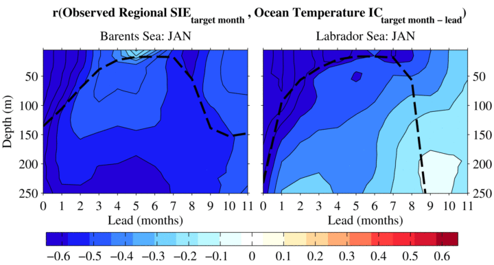 Correlation between observed regional SIE and regional-mean ocean temperature ICs in earlier months.
Correlations are plotted as a function of ocean depth and forecast lead time for the Barents and Labrador Seas and target month January. The linear trend is removed from both time series before the correlation is computed. The regional-mean mixed-layer depth climatology is plotted as dashed lines.
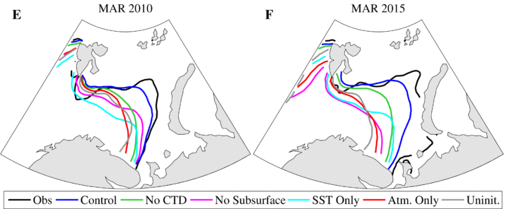 Predictions of the observed Barents Sea March sea ice edge (black) from the Control (blue), No CTD (green), No Subsurface (magenta), SST Only (cyan), Atmosphere Only (red), and Uninitialized (gray) OSE runs. Predicted ice edges for lead time of 8 months are shown for years 2010 and 2015.
Related Links
- September Sea Ice Outlook
- Sea Ice Prediction Network Web Portal
- Ensemble Kalman Filter Data Assimilation


