Operational Hurricane Track and Intensity Forecasting

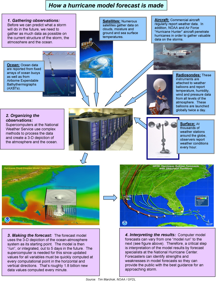
Over the past 20 years, significant advances have been made in the science of hurricane track forecasting. Much of this progress is due to advances in numerical weather prediction, that is, the use of computer models which approximate the fluid motions of the atmosphere to create forecasts of the weather at some time in the future. Since 1995, the GFDL Hurricane Prediction System has been used operationally by the National Hurricane Center and has consistently been one of the top-performing models utilized by NHC.

The challenge of representing a hurricane in a numerical model

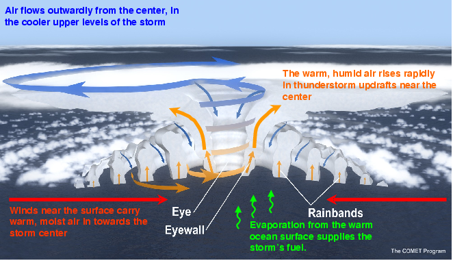
The atmosphere is a fluid of air parcels in constant motion. The laws of physics dictate the manner in which that motion takes place. Mathematical equations can approximately describe the various motions and interactions that occur in the atmosphere. One of the biggest challenges for hurricane modeling is creating a model that can accurately depict the large-scale, environmental flow of the atmosphere that is largely responsible for steering the hurricane, while at the same time representing the finer scale details of the inner core region that determine the intensity of the storm. The GFDL hurricane model is able to reproduce the features that are important in a hurricane. These include the inflow of low-level air into the hurricane’s inner core region; the supply of the storm’s energy from the evaporation of water from the ocean surface; updrafts of warm, moist air that feed thunderstorms in the core region of the storm, which help to intensify the hurricane; and the outflow of cooler, drier air at upper levels of the troposphere:

 

History of the GFDL Operational Hurricane Prediction System

The GFDL hurricane prediction system originated as a research model in the 1970s. The hurricane dynamics group at GFDL was formed under the leadership of Yoshio Kurihara for the purpose of performing hurricane research through numerical modeling. An axisymmetric hurricane model was constructed first, and then in 1973 experiments were made with a three-dimensional model. Throughout the next decade, many idealized numerical experiments demonstrated the capability of this model to produce a realistic hurricane structure, although it would not be until the 1980s that simulations would be attempted using data from real storms.

Results from real-data simulations and forecasts strongly suggested the potential of improving hurricane prediction with a comprehensive three-dimensional model. In the mid-1980s, GFDL scientists began a 10-year effort to transform their research model into an operational hurricane forecasting tool for the National Weather Service. Since becoming operational in 1995, the GFDL hurricane model has played a major role in improving hurricane prediction, resulting in a significant reduction in track forecast error.

Configuration of the model

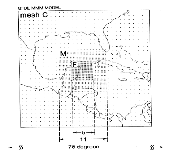
The current GFDL hurricane model is a gridpoint model that consists of three computational meshes which are nested together with increasingly finer grid-point spacing in each mesh. The size of the outer mesh is ~5000 miles wide with grid points spaced about 30 miles apart, while the finest mesh, where the grid points are spaced only 5 miles apart, covers a 325-square mile area. This area of fine resolution moves with the hurricane, keeping the storm centered in the middle of the innermost computational grid.

Coupling the atmosphere to the ocean in the hurricane model

In 1996, a collaboration began between scientists at GFDL and the University of Rhode Island (URI) to couple the atmospheric hurricane model to the Princeton Ocean Model. This coupling of the atmosphere with the ocean enables the model to reproduce the cooling of the ocean surface beneath the hurricane, which has an important impact on hurricane intensity. The GFDL/URI fully-coupled hurricane-ocean prediction system became operational in 2001. The research group at URI has also made important contributions towards improving the air-sea fluxes in the GFDL model.

 

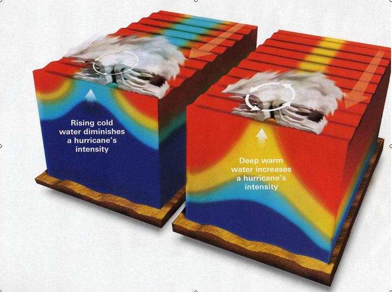
Hurricane-ocean interaction: A hurricane affects its own intensity by interacting with the ocean. The hurricane churns the water beneath it, bringing cooler water up to the surface from below and leaving a “cold wake” behind the storm. The cooler the water it brings up, the less fuel the hurricane has. When warm surface waters are shallow (left), cold water reaches the sea surface, greatly diminishing a hurricane’s intensity. Over deep warm waters (right), hurricanes have the potential to be more powerful because the ocean surface cooling is significantly less.

 

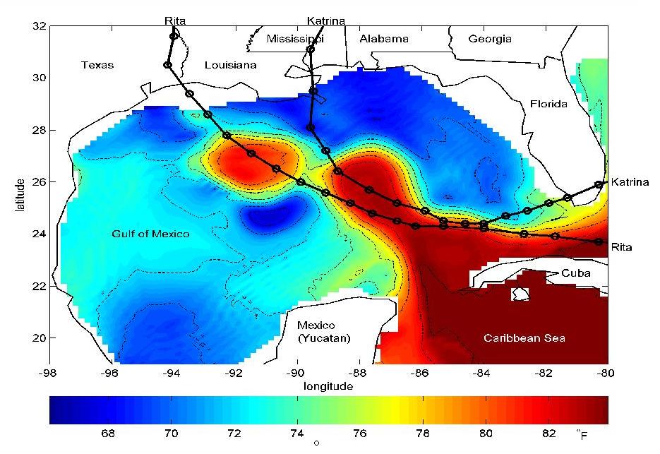
250 feet below the ocean’s surface: The above plot shows the temperature of the water in the Gulf of Mexico and northwestern Caribbean Sea in September, 2005, at a depth of 250 feet. The two black lines indicate the tracks that Hurricanes Katrina and Rita took as they traversed the Gulf of Mexico.  During Katrina and Rita, deep warm water in the Loop Current and within a Loop Current eddy was located under the storm tracks, which helped these storms to reach Category 5 intensity over the Gulf of Mexico. These ocean features are accounted for in the GFDL/URI coupled hurricane model.

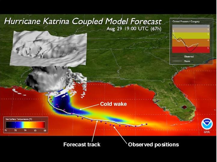
Forecasting Katrina: The above plot shows a snapshot from a GFDL forecast of Hurricane Katrina. The gray shading simply highlights portions of the storm structure (mainly the eyewall) by focusing on a particular level of equivalent potential temperature. This particular forecast was initialized 66 hours prior to landfall. As indicated, the forecast track was remarkably close to the observed track. Note the temporary decrease in magnitude of the cold wake in one area behind the storm, indicative of the passage of the storm over a region containing the deep warm water of the Gulf of Mexico Loop Current.

 

Upgrades to the Model

The GFDL hurricane model has been upgraded numerous times since it became operational at the National Weather Service in 1995.  In the following table, the major upgrades that have been implemented since 1998 are listed:

1998	Beta gyre in specified vortex replaced by asymmetries obtained from previous 12-h forecast Vertical distribution of target wind in vortex spinup made a function of storm intensity
2001	Atmospheric model coupled to a high-resolution version of the Princeton Ocean Model Upgrade of vertical diffusion from level-2.0 to -2.5 Mellor & Yamada closure scheme Effect of dissipative heating added
2002	Increase of horizontal resolution in outer nest from 1o to 1/2o Expansion of region covered by finest mesh (from 5o square domain to 11o) Modification of the filter that removes the global model’s vortex in the vortex initialization step (this upgrade enables more small scale features in the global analysis to be retained) Improved global vortex removal algorithm in initialization (less distortion of environmental fields)
2003	Increased vertical resolution (number of vertical levels increased from 18 to 42) Kurihara cumulus parameterization scheme replaced by Simplified Arakawa-Schubert (SAS) scheme Mellor and Yamada level-2.5 vertical diffusion scheme replaced by Troen and Mahrt (1986) Improved mass initialization for temperature and sea level pressure (reduced noise over mountains) Improved pressure gradient computation by using virtual temperature Effect of evaporation of rain included Further refinements to vortex removal algorithm in initialization More consistent target wind in vortex initialization Ocean coupling expanded to entire ocean domain Gulf Stream assimilation added to ocean initialization
2004	Introduction of one-dimensional ocean coupling in the eastern Pacific basin
2005	Addition of third nest with 1/12o resolution Improved vortex spinup with model physics consistent with the full 3-D model Elimination of mass initialization step
2006	Replaced the large-scale condensation scheme with Ferrier cloud microphysics package Improved air-sea momentum flux parameterization in strong wind conditions Assimilation of the Loop Current and warm-core eddies in the Gulf of Mexico added to ocean initial condition

 

Performance of the Model

In this section, we examine how well the GFDL hurricane model has performed throughout its years as an operational forecasting system.  The two components that are of the most significant importance to operational forecasters are track and intensity forecasting skill.

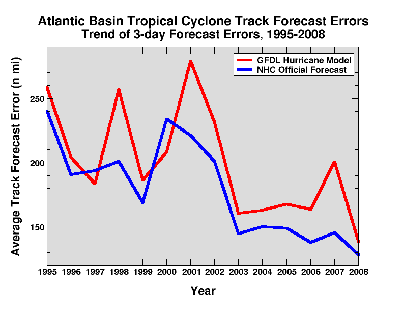
GFDL and  URI scientists have continued to transition the latest research advancements into the operational GFDL hurricane model, and this has resulted in a steady reduction in track forecast error since 1995.  The figure above shows a comparison of the 14-season trend of the 3-day track forecast errors for the GFDL hurricane model and the official forecast issued by the National Hurricane Center.  NHC uses the GFDL hurricane model as one of its main sources of forecast guidance.

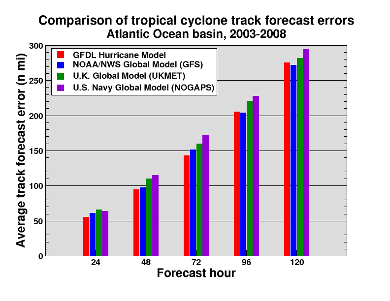
The figure above compares the average track forecast errors in the Atlantic Ocean basin during the past six hurricane seasons for the most reliable computer models available to the National Hurricane Center during this period.  The GFDL hurricane model had the most reliable track guidance and smallest track forecast errors through 3 days lead time and was near the top of the pack at 4- and 5-day lead time.

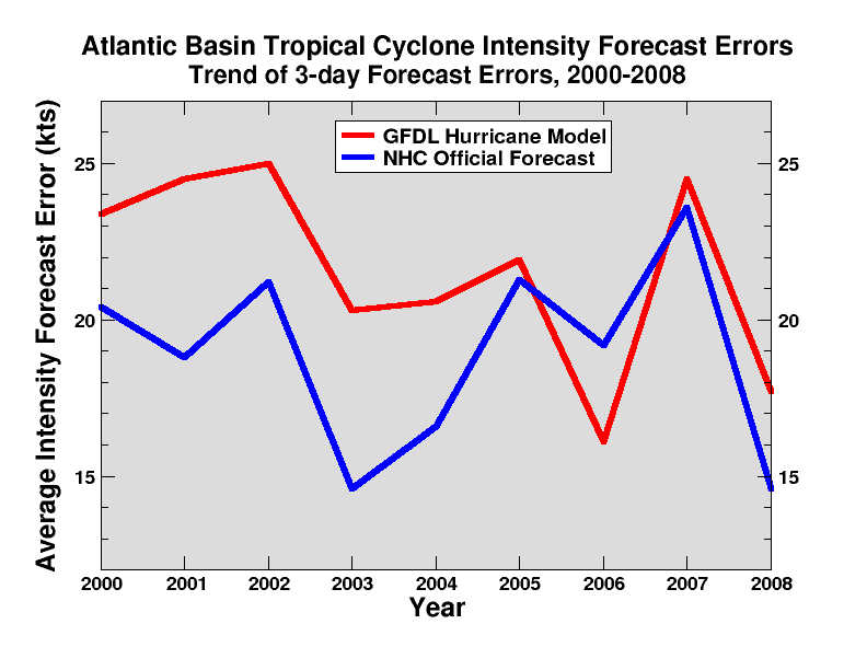
Until recently, even the most sophisticated dynamical weather prediction models were unable to provide skillful forecasts of changes to a hurricane’s intensity.  However, the latest upgrades to the GFDL hurricane model have led to significant improvements in hurricane intensity forecasts by better representing the atmospheric and oceanic physical processes critical for intensity prediction.  The figure above shows the trend of hurricane intensity forecast errors over the last nine seasons and even indicates that in 2006, for the first time ever, the GFDL hurricane model produced intensity forecasts that had smaller average errors than those from the National Hurricane Center’s official forecasts.

For more information, please contact Tim Marchok (Timothy.Marchok@noaa.gov)