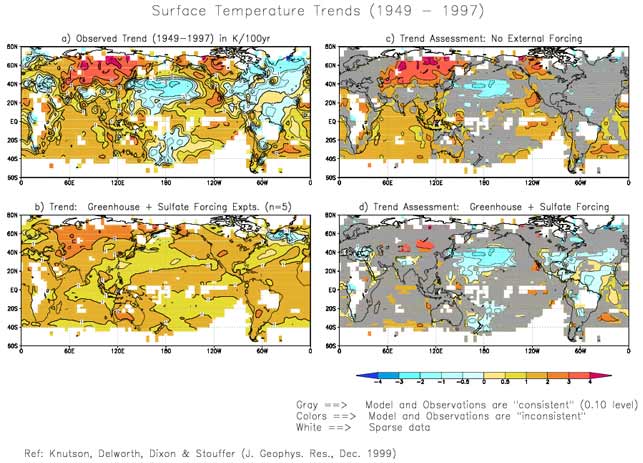
Simulated vs Observed Surface Temperature Trends (1949-1997)
Overview.
The diagrams below present evidence, based on model simulations and observations, that the recent surface warming trends in many regions around the Earth are likely due in part to a positive radiative forcing such as increased greenhouse gases. The warming trends appear to be particularly significant (panel c) in the Indian Ocean, much of Asia and western Canada, much of the eastern tropical Pacific, and the South Atlantic. On the other hand the cooling regions in the North Pacific, Northern tropical Atlantic, and Southeastern United States (panel d) are examples of regions where the observations are in significant disagreement with the model forced by greenhouse gases and sulfate aerosols. However, the model with greenhouse gas and sulfate aerosol (direct effect) forcings gives a better simulation of the past trends than the model without such forcings, as detailed below.
More detailed description: The figure below compares observed and simulated surface temperature trends for 1949 to 1997. (a) Observed surface temperature trend (1949-97) in degrees Celsius per 100 years. (b) Model simulated surface temperature trends for 1949-97 based on a greenhouse plus sulfate aerosol ensemble (n=5) experiment with the GFDL R30 coupled climate model. (c) Model assessment of the observed surface temperature trends in (a). Where plot (c) has gray shading, the trends are within the 90% confidence bounds of internal variability as estimated by the model. The remaining colored areas have trends that are “significant” in that they lie outside of this “natural internal variability” range. (d) Gray regions indicate where the observed trends in (a) and the simulated trends in (b) are “consistent” in that they are not significantly different from each other according to a t-test at the 10% level. The fact that a larger fraction of the globe is shaded gray in (d) than in (c) indicates that the trends in the greenhouse + sulfate aerosol runs are in better agreement with observations than are “internal variability trends” generated in the control run. Further details are contained in our JGR publication.
Click on the figure below to display a clearer image.


