

Posted on April 30th, 2012 in Isaac Held's Blog
 GISTEMP annual mean surface temperatures (degrees C)
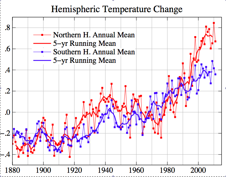
for the Northern and Southern Hemispheres.
Here’s an argument that suggests to me that the transient climate response (TCR) is unlikely to be larger than about 1.8C. This is roughly the median of the TCR’s from the CMIP3 model archive, implying that this ensemble of models is, on average, overestimating TCR
Formally, we define the TCR of a model by increasing the CO2 at the rate of 1%/year and looking at the global mean surface warming at the time of doubling. I have discussed the relevance of the TCR for attribution of 20th century warming and for warming scenarios over the next century in several earlier posts (3,4,6). Gregory and Forster (2008) – GF08 – is a good reference on this topic. The discussion below assumes that, for the time scales of relevance here, the forcing and response are more or less proportional with negligible time lag (i.e. 


The figure at the top of the post shows the time series of surface temperature averaged over the two hemispheres, from GISTEMP. The Southern Hemisphere (SH) has warmed relatively steadily over the past century, while the Northern Hemisphere (NH) warmed more rapidly in the first part of the century and from 1970-2000, with the familiar cooling episode in between. I expect the response to the WMGG’s to be roughly separable in space and time: A(t)B(x,y). One might conceivably see a slow drift in the pattern of the response, and some changes in structure near the sea ice edge, but it is hard to see how multi-decadal swings in the spatial structure could emerge from the forced response to WMGGs. GCM simulations are consistent with this expectation.
So this structure could be due either to the response to other forcing agents, aerosols in particular, or to internal variability. The major source of internal variability on these time scales is thought to be the pole-to-pole overturning circulation in the Atlantic ocean. Variations in the strength of this circulation alter the temperature difference between the hemispheres. In models, the mean NH temperature is a lot more responsive than the SH to this variability, so a stronger than average overturning warms the NH more than it cools the SH, resulting in a global mean warming and providing a consistent picture for the relatively steady SH trend. On the other hand, aerosol forcing is predominately located in the Northern Hemisphere, also providing a natural explanation for the relative shape of these curves to the extent that the time variation of the forcing matches features in the observed NH temperature variations.
It is important to sort out whether the non-WMGG forced response or internal variability is dominant in this regard, or if they both contribute substantially. But here I want to see what this plot implies about the TCR, irrespective of which of these sources is dominant. To do this, I am going to focus on the latest period, since 1980 or so, in which the rate of NH warming has been unusually large compared to that in the SH. Focusing on this most recent 30 year period has advantages because it is the satellite era, so we have more observations of things like total solar irradiance that help us reduce the mechanisms that we need to consider.
GF08 discusses the estimate of TCR that one obtains by making the simple assumption that neither internal variability nor aerosols affect the trend over the period since 1980. The WMGG forcing from 1980 to 2010 is 1.1 W/m2 using standard expressions (see this NOAA site), and is fairly linear in time. With a warming of 0.5K in global mean temperature 

GF08 use an estimate of the internal variability in 30-year trends (obtained from a GCM) to expand the uncertainty in this estimate beyond that coming from the regression itself; they assume that the system is equally likely to have been in a warming phase of multidecadal variability as a cooling phase over this period, so their uncertainty range remains centered around the TCR value of 1.8C.
But the rapid warming of the NH with respect to the SH over this 30 year period requires an explanation other than WMGGs. One possible explanation is that aerosol forcing has decreased over this period, enhancing NH warming. But if that is the case, the aerosol reduction is providing some of the global mean warming as well, so the total WMGG+aerosol forcing over this period would be enhanced, reducing the value of
By how much should we lower this estimate? You need to quantify and distinguish between the aerosol and internal variability sources to go much further. My personal best estimate is currently about 1.4C — I won’t try to justify this further here, but it is close to the central estimate for TCR in the recent paper by Gillett et al (2012).
A TCR of 1.4K corresponds to a value of 


It’s a simple story, based on a lot of assumptions. Analysis of GCMs with this argument in mind might help focus attention on aspects of model simulations that constrain TCR — or it might indicate weaknesses in the argument, allowing models to be consistent with the recent rate of warming in both hemispheres while simultaneously possessing a TCR larger than 1.8C.
[The views expressed on this blog are in no sense official positions of the Geophysical Fluid Dynamics Laboratory, the National Oceanic and Atmospheric Administration, or the Department of Commerce.]
Isaac,
It seems one of those many assumptions (that could be critical) is that the climate in 1980 was in equilibrium. In that case, part of the realized climate change since 1980 was a consequence of pre-1980 radiative disequilibrium.
Chris,
The assumption is not that the climate in 1980 is in equilibrium but that the heat uptake is proportional to the temperature anomaly from some (pre-industrial) equilibrium — ie. the system is in what I called the intermediate regime in post #3. (Actually post #4 — IH 5/17/12)
Isn’t that a very gratuitous assumption, especially since you do not take into account at all the ocean heat situation? In other words, all what you estimated was the maximum rate of warming towards equilibrium of the ocean + atmosphere in the current configuration!
As discussed by Gregory and Forster in the paper cited above, and in my paper with colleagues, and in several of my earlier posts, scaling the forcing by the TCR seems to work very well in emulating historical 20th century simulations in some GCMs. One way of thinking about this is in terms of a two-box model with very different heat capacities (or, more generally, a big gap between the characteristic time scales of the response of the ocean mixed layer and the rest of the ocean). If I understand you correctly, you are right that this assumption is effectively maximizing the heat uptake, since it treats the ocean beneath the mixed layer as an infinite heat reservoir — if you assume that parts of the ocean begin to saturate on relevant time scales, then the heat uptake would be reduced, holding everything else fixed. I wouldn’t call this “gratuitous” since I’ve been pretty explicit in previous posts about my reasons for exploring this simple assumption — but the existence of intermediate time scales in the response is very relevant to the question of how simple the relationship is between the forced response over the past 30 years and the forcing time series.
I used the therm gratuitous since without a very detailed analysis of the ocean temperature and very precise measurements of the outgoing microwave radiation (for which IMHO we do not have the full instrumental accuracy needed at this point) you can not seriously talk about estimating climate sensitivity.
I am not trying to estimate (equilibrium) climate sensitivity here. The whole point of focusing on TCR in this context is that, at least in the simplest picture, you don’t have to compute the strength of the top-of-atmosphere flux response and the heat uptake separately — you can try to constrain the sum of the two with the observations.
Isaac,
To expand on this in more words to make sure I understand-
There is a chance that the ocean continues to gain heat as it “attempts” to reach equilibrium with a “warmer than the little ice age but cooler than AGW” surface temperature + forcings system. If we held surface temperatures constant at 1980 levels we might see the ocean continue to warm for a while. This trend could extend to the present day and beyond, though it would decrease over time. Once the rate began to decrease significantly we would be out of the intermediate regime I guess. The additional warming trend from post-1980 GHG and other forcings could be superimposed on this pre-existing trend, though its curvature would likely be upward. (I am deliberately ignoring the fact that some of the pre-1980 trend would be due to GHGs).
Your choice of words, like “there is a chance” and “we might see the ocean continue to warm”, is not what I would use, since heat uptake observations and all climate models that I am aware of consistently predict substantial disequilibrium — but otherwise I think we are on the same page. If the forcing increases linearly in the future, so that the fast response is also linear, then one should expect some upward curvature in the forced response as warming of the deep ocean due to past forcings takes hold, and the surface warming is not held back as strongly by its coupling to deeper layers. As always, internal variability is superposed on this forced response.
I am curious what the hemispheric difference in the rate of ocean heat uptake would add to this discussion. From Levitus et al 2012, since 2005 & extended until mid-2012, it appears the oceans (0-2000m depth) have warmed at a rate of about 0.7 W/m^2 globally, but the NH rate is 1.5 W/m^2 while the SH rate is more than an order of magnitude lower and more or less indistinguishable from zero. Of course this is a very short time period, but the NH rate is strongly consistent over this period (R^2 for OLS – 0.7).
In the context of this post, I doubt that a focus on such a short period can help us constrain the TCR in the absence of a rather precise understanding of what the internal variability is up to. Levitus et al does show substantial SH heat uptake in the longer term trends in their Fig. 3. But more generally I agree that the differences in heat uptake between the two hemispheres can affect the kind of argument that I am referring to in this post. You can change the differential warming by changing the differential heat uptake — the atmosphere does not mix efficiently enough between hemispheres to make you insensitive to these differences in uptake.
I’m surprised not to see more literature on the hemispheric differences than what I’ve encountered on brief searches. I found an interesting paper, perhaps never published (here), “Croll Revisited” by Kang and Seager. This paper attempts to build on Trenberth and Fasullo 2008 (here). T&F’s Fig 2 shows a net energy flux from ocean to land, via the atmosphere; Kang and Seager show a smaller net energy flux from SH to NH via ocean heat transport. This may agree with the statement in your post that GCM’s show some hemispheric difference although not as much as in the past 30 years. In other words, I guess I am coming to terms with your sentiment that some hemispheric difference simply due to a forced response would be expected.
Hi Isaac,
Nice post. What if a devil’s advocate argued that the reduced temperature trend in the SH could be a forced response? E.g. both ozone depletion and increasing NH aerosols are known to cause large SH circulation changes in some GCMs, and I could imagine that this in turn could result in significant radiative forcing?
Or does the relative linearity of the SH trend compared with the NH trend make you think that any forcing beyond WMGG must be impacting the NH more than the SH?
Joe,
Does the stratospheric ozone hole cool the SH surface as a whole?
I am sympathetic with your last sentence.
would it not be easy to check the TCR of the cmip5 models which can reproduce the observed pattern of historical warming (e.g. Booth et al. 2012)?
Do these models have a lower TCR than the rest of the ensemble? If so then you have a nice explanation as to why here… Perhaps that is what you are proposing.
Exactly — and if models that fit the NH/SH differential warming best do not have TCRs lower than 1.8C or so, we learn something (or at least I do) by seeing where this argument breaks down.
Isaac – Thanks for a thought-provoking analysis. The paper by Zhang et al (you’re the senior author) was very useful in elaborating on the concepts and discussing some of the uncertaintites. One question that comes to mind is this – to what extent is what you describe as “internal variability” that might contribute to a net warming via the NH/SH differential a forced response to GHGs?
Fred,
How plausible is it that well-mixed greenhouse gases in isolation could have forced the very different warming trends in the NH and SH over the past 30 years? Shouldn’t we expect WMGG-forced warming to be larger in the NH? Yes, but a factor of 2? I have assumed that this is implausible, but I need to return to this in another post to support this claim.
I am interested by the radiative restoring implied by your personal TCR estimate of 1.4 K. As you write, the radiative restoring
 is consistent with the fixed relative humidity feedback with no cloud feedback. But estimates of cloud feedbacks in the CMIP3/AR4 models are generally positive: both in the multi-model mean and basically every individual GCM [e.g., Soden and Held (2006). Are similar feedback analyses available for CMIP5 GCMs?]. How can your argument and expectations based on comprehensive GCMs be reconciled?
Tim,
If you are going to try to argue, from a holistic perspective, that the CMIP ensembles overestimate TCR on average, then you are probably going to have to argue, from a reductive perspective, that the cloud feedback is contributing too much to the warming in the models.
Isaac – A study similar to GF08 was Padilla et al 2011, which used a Kalman filter to recursively narrow the TCS (transient climate sensitivity) range when applied over the twentieth century, and arrived at a most probable TCS (similar to TCR) of 1.6 C and a range of 1.3 to 2.6 C. These values varied somewhat when uncertainties in forcings and/or natural variability were included.
I’m interested in your evaluation of their method and results, including the wide range and upper limit they estimated.
One difference is that Padilla et al focus on the global mean only. They do point out that focusing primarily on the most recent period does reduce their TCR estimate. (And a lot in a study like theirs depends on the aerosol forcing range.) I guess my main point, and that of Gregory and Foster and some of the other papers mentioned in the post) is that it is valuable to focus on this recent period. Although it is not clear from what I have said here, there is the hope of bringing a much larger diversity of data into the argument in this later period– TOA fluxes, patterns of ocean heat storage etc — than for the century as a whole. But the shorter the period, the more you have to focus on internal variability.
Isn’t most of the difference between the NH and SH trends due to changes in the arctic? I think 0-60 degrees N would look very similar to 0-90 degrees S. You seem to offer several possible explanations for the difference between the two hemispheres. If the difference is mainly in the polar changes which explanation does that favour?
Nice post BTW, it’s got me thinking. I actually wanted to ask something about cAGW but I suspect those sorts of questions are bypassed on this blog???
Perhaps someone with a few minutes of spare time (unlike me today) could check how much the plot at the top of the post is affected by truncating the average at 60N-S.
Tried to get this as close to the original graph style as possible, for comparison: .
Using the indispensable http://climexp.knmi.nl/ I get 0.2ºC/Decade for 0-60N and 0.08ºC/Dec for 0-60S. Using NOAA’s analysis I get 0.21ºC/Decade for 0-60N and 0.09ºC/Dec for 0-60S.
The polar regions (defined as 60-90º) have trends of 0.6ºC/Dec and 0.08ºC/Dec for North and South respectively. However in NOAA’s analysis the figures are 0.37ºC/Dec and -0.05ºC/Dec.
It’s also possible that the increased NH trend is due to greater albedo feedback in the NH with the loss of Arctic sea ice and NH snow cover. Given that the Arctic is one of the most rapidly warming regions, this seems plausible. In that case, ξ has been estimated correctly at 1.8, and 1.4 may well be too low.
Whether it is due to the Arctic or the land/ocean fraction (I suspect the latter is more important) the question is whether WMGGs in isolation can force this large an interhemispheric difference in warming. If they can, then one could argue that it is only in this latest period that the WMGG signal is emerging clearly and that, say, over the century as a whole the NH warming has been held back by aerosols. This is one way of arguing for a TCR range centered on 1.8K or so.
You may find this plot of GFDL’s CM2.1 output for the 1% to doubling run useful:
source data:
My impression is that CM2.1 has one of the smaller NH/SH ratios of warming in the 1%/yr simulation of any of the CMIP3 models — but I do not have the results handy to back that up.
Having only explored the GFDL portal I don’t know either.
I did take a shot at comparing the 20th century CM2.1 runs to GISTEMP on a latitude basis. My attempt to recreate the global annual T anomaly from the model runs and compare to GISTEMP is here:
My comparison of the decadal average anomalies by latitude between the average of all 5 model runs and GISTEMP is here (model runs are anomalized to 1950-1980 to match GISTEMP anomalies):
The way I read the latter plot is that large differences in the latter decades between CM2.1 and GISTEMP could be the result of differences in the 1950-80 period or differences since. If I combined the 1950-80 curves for either the model or for GISTEMP they would be flat lines at zero at all latitudes.
I should say for anyone else reading this, I have no real understanding of how the model works; I am just playing with the output.
One add-on thought is that Isaac or somebody else familiar with this particular model would be able to determine if the ensemble mean global anomaly (black line in the first figure) looks right compared to GISTEMP; for example the apparently exaggerated cooling in volcano years.
The possibility that models are over-emphasizing the volcanic responses is something that a number of people are looking at — but you have to be careful — the ensemble mean will always show the volcanic signal more clearly than individual realizations.
Issac,
Regarding Heat Uptake Efficiency (gamma) I can only refer back to earlier simpler models such as the Upwelling Diffusive Ocean and what you gave us in post number 4 “Transient vs equilibrium climate responses”. My thoughts are hence not novel but I will give them anyway.
The efficiency has the units of a thermal admittance (flux proportional to temperature), the only component that corresponds directly to the this seems to be due to the vertical circulation ~4m/year averaged over the oceans which corresponds to ~16MJ/m^2/yr/ºC ~ 0.5W/m^2/ºC over 70% of the globe ~ 0.35W/m^2/ºC if the warming is even.
The potential for changes in heat flow due to perturbation of that mass flow seems considerable due to the large difference between mean SST and abyssal termperature say ~12ºC (to pick a figure) or ~0.04W/m^2 for a 1% perturbation of the mass flow.
If I recall correctly, probably from Walter Munk (Abssal Recipes?) the effect of such perturbation is a bit paradoxical. The general whole ocean upwelling is viewed as returning heat that is diffusing down (relative to the moving column) back to the surface, e.g. a slowing of the vertical ascent of cold water would cause an uptake of heat or put the other would reduce the rate at which heat is returned towards the surface. Locally over generalized upwelling areas that are net exporters of ocean heat this uptake should be associated with increased SST due to the lessening of that exportation, which seems decidedly odd.
The uptake due to the heating of the WML is a function of dT/dt not T so once the dT/dt has stabilized it doesn’t contribute to gamma which leaves only the change in the perturbed diffusion heat flux rate. Again this is not a function of T but closer I think 1/Sqrt(T) for a steady dT/dt so it is potentially large in the initial transient. In this case the timing of that transient would likely have been determined by the pre WWII warming as it relates to thermal perturbation stretching down through the top ~1km of the column. If that is the case although the total perturbed flux may be substantial by now, its change during the recent warming is likely to be only the minor fraction of that. My best guess (but only that) would be for a similar figure of ~ 0.35W/m^2/ºC. That said I think a decent figure could be estimated from the SST history and estimates of the effective vertical diffusion coefficient.
Totaling up one would have ~0.7W/m^2/ºC. Plus or minus 0.04W/M^2/ºC per 1% perturbation of the mass flow. The effect of the mass flow should probably be integrated and then averaged if the perturbation is thought to be changing in time and hence temperature.
I do not know what figure people might say were plausible for a slowing of the mass flow but if it can really be viewed as an whole ocean effect it would have a general cooling effect proportional to the amount of ocean of which there is about 1/3 more in the SH than the NH favouring less southern warming but also a reduction in the Equator to Artic flux favouring less northern warming but that might be taken up by increased atmospheric flux as I think it be the total that is governed and that to be approximately equal in both hemispheres.
If the NH (I suppose mostly Artic) downwelling is disproportionately large compared to the SH that would increase gamma due to the higher NH and Artic warming rate but would make that same warming more difficult to explain.
In many respects the two hemispheres are rather similar. From an old data table (Sellars 1965) I read that the hemisperic means for altitude (helped by Antartic Plateau), temperature, rainfall, evaporation, precipitable water, cloud and albedo have little to distinguish them. There is ~ twice as much land in the NH but put another way the SH only has about 1/3 more ocean. What is true is that the poles are distinctly different in altitude and temperature but that I think is only one independent difference and one dependent one.
Alex
Routing through more of the Climate Explorer information, one realisation of the HadGEM2-ES model appears to have a very similar hemispherical contrast. According to this document it has a TCR of 2.5K.
This clearly looks like an interesting model vis a vis the argument presented here.
This model has a 1900-2004 temperature rise of only 0.22 C (compared with the observed 0.74 C), a strong mid-century cooling, and an estimated ECS (preliminary) of about 4.5 C. I have the impression that it may have overestimated negative aerosol forcing, at least compared with the other models.
It’s the same model as the one used for the recent Booth et al. Nature paper on Atlantic aerosol effects.
In “WMGG”, what do “WM” stand for?
Assuming (something not known) that the current reduced or non-warming persists for 20 more years (I did say this was a counterfactual hypothetical), how does that alter your estimate? In the Padilla et al paper the authors wrote that the next 20 years should produce a great reduction in the uncertainty of the estimate of tcr; what would this particular trend that I hypothesized produce in the point estimate itself?
I can appreciate if you think this is an idle speculation.
Matt – Your substantive question was addressed to Dr. Held, but regarding the abbreviation, WMGG stands for well-mixed greenhouse gases (CO2, methane, etc.)
“Well-Mixed” – and, therefore, long lived (LLGG is another acronym often encountered) — to distinguish from water vapor, ozone, etc.
As for the question about the next 20 years, I think the key will be to actually understand what is going on — from spatial structure, TOA fluxes, the pattern of the ocean heat storage, aerosol measurements. Of course 20 more years of data will help a lot, but I suspect that we could do better in constraining TCR right now.
Dear Prof. Held,
I have noted your earlier comments about undue focus on equilibrium climate sensitivity (ECS). However, this is the metric people are most familiar with and may assist in comparing your estimate and Gillett et al. with other estimates.
In the IPCC AR4,
“… it can be estimated that in the presence of water vapour, lapse rate and surface albedo feedbacks, but in the absence of cloud feedbacks,
current GCMs would predict a climate sensitivity (±1 standard deviation) of roughly 1.9°C ± 0.15°C”.
I note this value is similar to what Schwartz (2012) has also just found. Given that you’ve said your best guess of TCR is similar to a constant relative humidity model with no cloud feedback, can I take that to mean you also agree that ECS might be something like 1.9 K ± 0.15°C?
(Note I am not the same person as Alexander Harvey above.)
I don’t think that the warming over the past few decades, or the past century, constrains equilibrium sensitivity very strongly. I have tried to argue in previous posts that the connection between the transient and equilibrium responses may not be as tight as one might think based on the simplest energy balance models. Different processes can come into play on long time scales with different spatial structures in the surface temperature response and different feedbacks. So i am going to try to keep the focus here on TCR.
Dr. Held,
Very interesting post. Not sure if you’ve already crunched the numbers for the CMIP5 models for a subsequent post, but a quick analysis using the CMIP3 models (from Climate Explorer) yields the following results for me (TCR from AR4 WG1 table 8.2):
http://i.imgur.com/esidoUt.png
which seems to indicate that none of the models quite duplicate the NH trend / SH trend ratio of GISSTemp. However, the models with multiple runs show that natural variations can impact this ratio a good amount over this time period (particularly in GISS-EH).
Running a simple regression on the two variables (average trend + NH/SH ratio) may have some predictive power with respect to the TCR (r^2 ~ 0.15%), and plugging in those values for GISSTemp would seem to indicate a likely value for TCR of about 1.4 K you suggest, although the uncertainty is quite large.
Thanks — Before trying to understand this aspect of the models 20th century simulations, I would like to have a better feeling for the NH/SH warming ratio in CO2 only (1%/yr) simulations, since the starting point for the argument above is that it is hard to get the observed ratio with greenhouse gas forcing only. (I probably won’t be checking in on the blog much in the next week.)
Perhaps noteworthy as an additional reference, UAH reports NH/SH = 2.7 and global trend = 0.13, lower than GISTEMP but slightly higher than the highest model. Sure it’s not quite the same variable but shows a similar pattern. Troy do you know how possible it is to crunch the CMIP5 runs in a similar fashion?
A slightly off beam question:
Is it a necessity that all forcings (w/m2) must have the same temperature impact?
I ask because a transient climate sensitivity derived using the ‘sum of all forcings’ from 1980 to 2010 would seem to be incompatible one derived from the period 1910 to 1940.
This question is not off beam at all. The temperature response per unit radiative forcing can be different for different forcing agents — we say that they have different “efficacies”, which is just a fancy way of saying the same thing. But more importantly, there is real danger of overfitting by trying to match forcing and response over time in detail. This would be OK if you had multiple realizations of the 20th century and could then remove the effects of internal variability by averaging, isolating the forced response, but we only have one realization of nature. For the recent period, a lot of evidence points to a modest but non-trivial positive contribution to the warming from internal variability, and as suggested in the post, I would try to take this into account when trying to estimate TCR from this period. For the earlier period, with a lot less evidence, I suspect that that internal variability played some role as well, but its going to be a lat harder to quantify than for the recent warming period. Other things to worry about: How well do we know the forcing? and am I oversimplifying things by implying that the TCR concept can be applied quantitatively in this simple way, since this depends on there being a sharp distinction between fast and slow climate response times?
My apologies for the lateness of this comment. I have only just studied this post in detail, having been prompted to do so by a tweet from Andrew Revkin. I note that you derive an upper limit for TCR of 1.8 K. I won’t query your method, but I don’t think your calculations are correct. You say:
“The WMGG forcing from 1980 to 2010 is 1.1 W/m2 using standard expressions (see this NOAA site), and is fairly linear in time. With a warming of 0.5K in global mean temperature T, this would require a value of ξ (in T = ξ F) of about 0.45C/(Wm-2). … A value of ξ = 0.45, multiplied by the standard CO2-doubling forcing of 3.7 W/m2, gives a value of about 1.8C for TCR.”
Two points:
1) 0.45 x 3.7 = 1.665 , not 1.8. A slip of the calculator, perhaps?
2) The change in global mean temperature from 1980 to 2010 appears to have been less than 0.5 K. Per a recent download of GISSTemp, the rise was 0.44 K. Per a recent download of HadCRUT4, it was 0.447 K.
The HadCRUT4 figure is higher than that per HadCRUT3, which was 0.400 K. The 1980-2010 temperature increase per NOAA-NCDC is 0.428 K. Per the Japanese Meteorological Agency record it is 0.32 K.
The average of the HadCRUT4, GISSTemp, NOAA-NCDC and JMA rises is 0.409 K.
Since JMA is an outlier (but could be correct – they have much experience in measuring sea surface temperatures in particular) I will treat it separately. Substituting HadCRUT3 for JMA, the rise would be 0.429 K.
Adjusting for the erroneous multiplication and surface temperature rise data, the implied upper limit on TCR based on the average of the HadCRUT4, GISSTemp, NOAA-NCDC and HadCRUT3 temperature rises is then calculated as:
ξ = 0.429 K / 1.1 = 0.390, and TCR_max = 0.390 * 3.7 = 1.443 K
Based just on GISSTemp, the record shown in the graph, one gets:
ξ = 0.44 K / 1.1 = 0.40, and TCR_max = 0.40 * 3.7 = 1.48 K
Based just on the JMA record, the calculation is:
ξ = 0.32 K / 1.1 = 0.291, and TCR_max = 0.291 * 3.7 = 1.076 K
Even if one took the fastest rising of the five surface temperature records, HadCRUT4, on its own, TCR_max would only come out as 1.50 K.
Do you agree that the calculation of TCR_max as 1.8 K was in error?
It is also interesting to compare these corrected estimates with a TCR corresponding to the well-constrained estimate of 1.62°C for effective/equilibrium climate sensitivity that I recently derived using a heat balance method almost identical to that in Gregory et al., 2002 (details at webcitation.org/6DNLRIeJH ). My calculation was based on mainstream observational estimates for changes in temperature, forcings and ocean heat uptake (OHU), and underlay the estimate given in a Wall Street Journal article by Matt Ridley in December. The corresponding TCR depends on how one treats OHU, but is of the order of 1.3 K. Going the other way, a TCR_max of 1.44 C corresponds to an upper limit on effective/equilibrium climate sensitivity of circa 1.8 C, assuming (modest) OHU consistent with observations.
By this method, TCR . With T = 0.5,
  , and
, and  you get TCR = 1.68. If you use the actual value for the WMGG forcing over this 1980-2010 period from the NOAA site (1.044), you get something that can legitimately be rounded to 1.8K. (This might be what I actually did, and then evidently rounded inaccurately when I wrote the post.) If you use the linear trend over this period from GISS, rather than the endpoints that I think you are using, you get T a bit larger than 0.5, so I am not sure that I need to revise this TCR_max estimate. In any case, the forcing is the key uncertainty if you ignore internal variability– can one really avoid aerosol forcing by choosing the time interval in this way, plus there are the minor but not negligible forcings like the solar cycle TSI and stratospheric water.
I’ll avoid the question about equilibrium sensitivity for the moment — I hope to return to it soon (if I can find the time to post at all). But TCR is a more direct way of projecting global mean temperature for the next 50-100 years, given the forcing. I don’t think estimates of equilibrium or “effective” sensitivity add much if this is the main objective.
Thank you for responding.
Yes, I did indeed use the endpoint GISS etc. temperatures, as there was no indication that the linear trend had been used rather than the actual temperatures. I can see arguments for using either here.
I have noticed, incidentally, that the GISS estimate of the WMGG forcing increase over 1980-2010, at 1.264 W/m^2, is far higher than that per NOAA at 1.044 W/m^2. But GISS is an outlier, I think.
I should have said in my comment that I found your arguments as to why this method provided a maximum estimate for TCR interesting. I realise that argument was the main point of the post, not the particular numbers.
One of the problems that I see with using TCR is that it is quite strongly dependent on the period over which it is measured, if diffusive ocean heat uptake is significant. That is one reason for preferring to work with equilibrium/effective climate sensitivity (or its reciprocal the climate feedback parameter) and effective ocean vertical diffusivity. Those parameters seem more closely related to the approximate large scale physics of the climate system, and are (at least as a first approximation) independent of whether thay are taken over (say) 30, 70 or 100 years. TCR over any period can be derived from those parameters (together with the mixed layer depth). Maybe you are ignoring time-dependence of TCR because in a simplified 2-box ocean model with a shallow mixed layer TCR is nearly independent of timescale.
“Diffusion”, by which I interpret you to mean vertical diffusion, is not how the oceans or ocean models actually take up heat — whether it is a useful surrogate for what is actually going on is not obvious. The two box model does a pretty good job of mimicking GCMs (see Geoffroy et al, 2012). But, ignoring issues related to internal variability, the TCR estimate based on 1980-2010 should be an underestimate of the classically defined TCR if there is appreciable saturation of the deep ocean sink on multi-decadal time scales. (Revision: with a clearer head a few hours after posting this, I need to retract the previous sentence. If one is just sampling, over a short time span, the forced evolution due to evolving forcing agents that are characterized by longer time scales, one is not biasing the estimate of TCR due to an overestimate of heat uptake — it is only an underestimate of TCR if the forcing has time scales comparable to the short time window you are looking at — sorry .) The value of the classically defined TCR is that it is readily available from models, helping us judge their sensitivity. For the CM2.1 model discussed in a number of previous posts in this series, one can see that this saturation is negligible at present in those simulations by looking at what some of us call the “recalcitrant warming” — post #8.
I think your estimate is way to high due to ENSO and AMO.
Forster/Rahmstorf do a regression with the ENSO index but the ENSO index is in no way linear to the temperature effect of the ENSO process. The main difference is due to the aftermath of El Nino events, whereby warm water pools drift out of the index region and continue to warm for years.
It would be therefore much better to use start and end points, where PDO and AMO have been in very similar states, such as 1945-2005.
If you do that, you will arrive around 1.02K transient (and about 1.65K equilibium)
https://web.archive.org/web/20130129012549/https://judithcurry.com/2013/01/25/open-thread-weekend-7/
And possibly further reduction with new estimates for black carbon.
I think you may have misunderstood my post which was at least in part about the possibility that the AMO could, as you mention, create a high bias in the estimate of TCR based on this period. The problem with the longer time span that you suggest for an analogous analysis is that it becomes much harder to avoid the need to estimate aerosol forcing.
Dear Prof. Held,
I see in your post above you assumed a heat uptake efficiency of 0.7 W m-2 K-1. And I note your comment about wanting a simple theory for the number.
I was reading a paper by Stephen Schwartz –
Determination of Earth’s transient and equilibrium climate sensitivities from observations over the twentieth century: Strong dependence on assumed forcing. Schwartz S. E. Surveys Geophys. 33, 745-777 (2012). DOI 10.1007/s10712-012-9180-4.
https://www.bnl.gov/envsci/pubs/pdf/2012/BNL-96153-2012-JA.pdf
In this paper the author has claimed that to the best of his knowledge he has made the first observational estimate of the heat uptake coefficient in the literature, and he finds a value of 1.05 +/- 0.06 W m-2 K-1. He notes this is somewhat larger than in the GCMs.
I just wondered if you had any thoughts on his estimate or on how much this might affect your analysis.
Kind regards,
Alex Harvey
Alex, the link didn’t work for me but the paper is easily located from Schwartz’s home page. I’ll defer comment on the paper itself till I have had time to read it carefully. Just to re-iterate, there is no need to refer to the value of the heat uptake efficiency when estimating the TCR by these simple top-down methods.
I am getting a little worried that I may be contributing to an over-obsession with these analysis of the global mean time series. I doubt that the heat uptake in the Southern Ocean, for example, has much effect on the warming in the Northern Hemisphere. Yet if all you’re doing is working from this global mean picture, you might be misled into thinking that it does.
Isaac – Sorry to belabor the TCR issue again, but AR5 has focused renewed attention on it. The work of Martin Wild and others on global dimming and brightening implies that reduced aerosols after 1980 contributed to the positive forcing. My question is this: over the short term (a few decades or less), how effective are aerosol forcing changes in driving temperature changes compared with WMGGs? The NH/SH difference is consistent with aerosol effects at least temporarily acting disproportionately over land compared with WMGGs. Wouldn’t land warming or cooling be relatively deficient in its ability to alter radiative restoring via feedbacks from water vapor, clouds, and the melting of sea ice? If so, might net positive forcing since 1980 underestimate the ability of similar forcing by CO2 alone to elevate temperatures? Has this been looked at anywhere?
Since asking my question, I’ve seen a recent paper by Chin et al Multidecadal Variations of Atmospheric Aerosols that reports aerosol optical depth to have changed little globally from 1980 to 2009, but to have shifted geographically. Europe, North America, and Russia have seen a reduction, while some regions further south in the NH and a few south of the equator have seen increases. Perhaps this could explain at least part of the diverging NH/SH trend without requiring a major positive forcing change from aerosols.
Fred,
I think your impressions on this issue are as good as mine. These geographical changes in the aerosol loading make it more challenging to separate the WMGG, aerosol, and internal variability components from the observed evolution of the full temperature field. Unlike WMGGs, we presumably can’t assume that there is just one spatial temperature pattern that corresponds to the aerosol forced response, something that fingerprinting studies need to take into account . One also has to worry about the mix of absorbing and scattering aerosols changing in space and time. i don’t have any special insights on this. I suspect that the radiative forcing concept, as an intermediary between the aerosol distributions themselves and the climate response, is a lot less useful here than for the WMGGs, especially when one gets down to the effects of changing spatial distributions and cloud-aerosol interactions.