46. How can outgoing longwave flux increase as CO2 increases?

Posted on May 31st, 2014 in Isaac Held's Blog

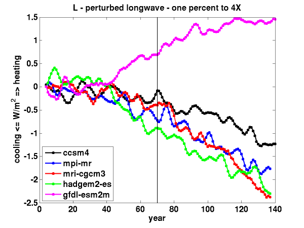
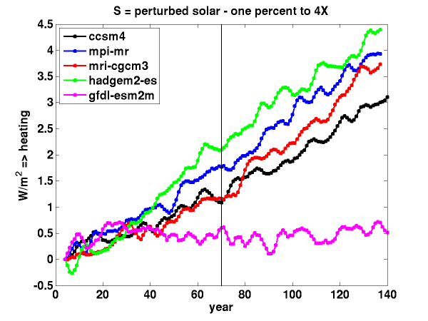
Evolution in time of fluxes at the top of the atmosphere (TOA) in several GCMs running the standard scenario in which CO₂ is increased at the rate of 1%/yr until the concentration has quadrupled.

A classic way of comparing one climate model to another is to first generate a stable control climate with fixed CO₂ and then perturb this control by increasing CO₂ at the rate of 1%/yr. It takes 70 years to double and 140 years to quadruple the concentration. I am focusing here on how the global mean longwave flux at the TOA changes in time.

For this figure I’ve picked off a few model simulations from the CMIP5 archive (just one realization per model), computed annual means and then used a 7 yr triangular smoother to knock down ENSO noise, and plotted the global mean short and long wave TOA fluxes as perturbations from the start of this smoothed series. The longwave ( $L$ ) and shortwave ( $S$ ) perturbations are both considered positive when directed into the system, so $N = L +S$ is the net heating. The only external forcing agent that is changing here is CO₂, which (in isolation from the effects of the changing climate on the radiative fluxes) acts to heat the system by decreasing the outgoing longwave radiation (increasing $L$ ). But in most of these models, L is actually decreasing over time, cooling the atmosphere-ocean system. It is an increase in the net incoming shortwave ( $S$ ) that appears to be heating the system — in all but one case. This qualitative result is common in GCMs. I have encountered several confusing discussions of this behavior recently, motivating this post. Also, the ESM2M model that is an outlier here is very closely related to the CM2.1 model that I have looked at quite a bit, so I am interested in its outlier status.

Since the radiative forcing due to CO₂ is logarithmic over this range, the radiative forcing increases linearly in time. Global mean surface temperatures $T(t)$ also increase roughly linearly in time, as does the heat uptake $N(t)$ , as seen in the following:

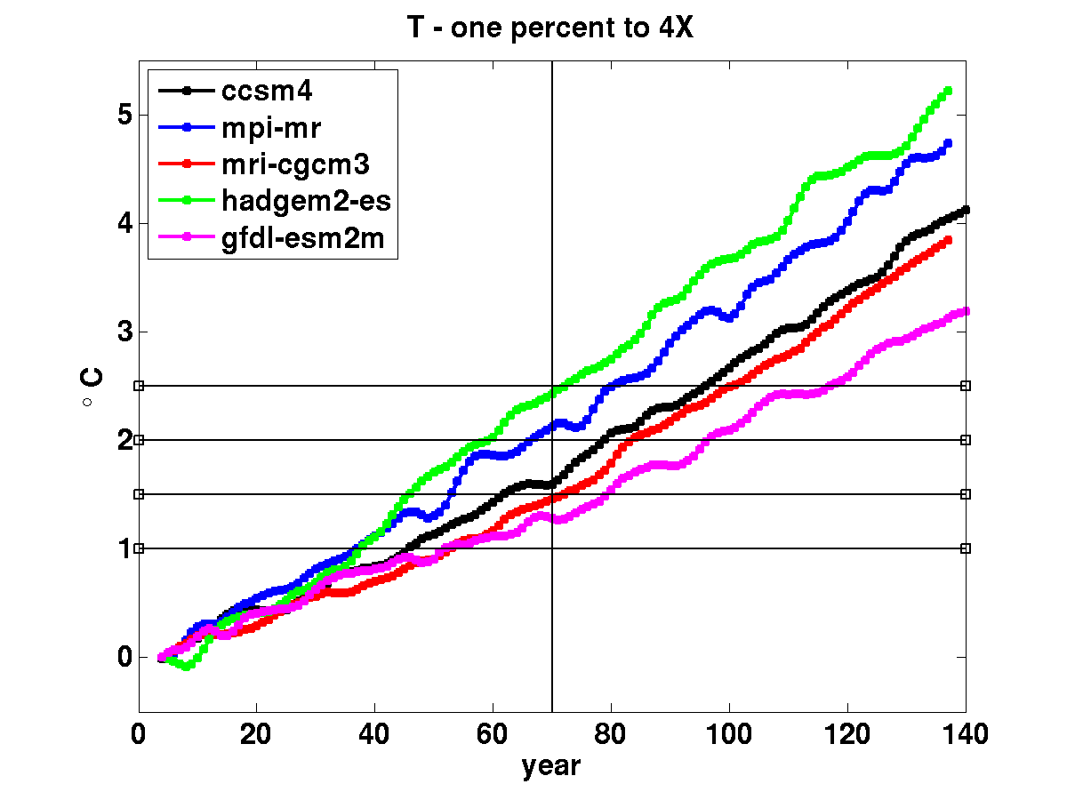
Another reason that I am interested in this comparison is that ESM2M has a low transient climate response ( $\approx 1.3C$ warming at the time of doubling) that I like for a variety of reasons.

When thinking about this sort of thing, I tend to start with the energy balance of the ocean mixed layer, the surface layer of the ocean that is well-mixed by turbulence generated at the surface. Globally averaged we can think of this layer as being something like 50m deep, providing a heat capacity that is more than an order of magnitude larger than the atmosphere. Ignoring the latter, we can think of $N = L + S$ as heating this layer directly. This surface layer is cooled by transfer of heat $H$ to deeper layers of the ocean:

$c \frac{\partial T}{\partial t} = L + S - H$

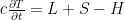
On the time scales of interest here the heat capacity of this layer is itself negligible and we can ignore the time-derivative in this equation, so that 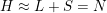$H \approx L + S = N$ . For small perturbations, I’ll assume that $L = F_L - \beta_L T$ where $F_L$ is the CO₂ forcing and $\beta_L$ is the sensitivity of the longwave flux to temperature. We could also write $S = F_S - \beta_S T$ in general, but in this case of CO₂ forcing only , $F_S$ is small and we can think of $S$ as pure feedback.

Importantly for this discussion, I am also going to write $H = N =\gamma T$ . $\gamma$ is referred to as the efficiency of the heat uptake — the heat uptake per unit global warming. This allows us to define a transient climate response very easily — solving for $T$ :

$T = F_L/(\beta_L + \beta_S +\gamma)$

In previous posts, I have referred to the time scales of the forcing for which this is a useful first approximation as the intermediate regime (this hasn’t caught on — maybe I should try something else) — intermediate between the faster time scales (due to volcanoes for example) for which the heat capacity of the mixed layer is important and the slower time scales over which the deeper ocean starts to equilibrate.

With these sign conventions, $\beta_L$ and $\gamma$ are positive, while $\beta_S$ is negative if shortwave feedback is positive (sorry). If all of these coefficients are constant in time over these 140 years of simulation, and given our other approximations, we expect $T$ and $H$ to both increase linearly in time, as is roughly the case in these models. (Actually, $T$ is typically a bit concave upwards while $H$ is a bit concave downwards, but I think the simplest model is adequate here even if it can only fit these curves to the extent that they are linear in time.) Solving for $L$ ,

$L = F_L - \beta_L T = F_L (\beta_S + \gamma)/(\beta_L +\beta_S +\gamma)$

Whether $L$ increases or decreases in time — that is, whether the forcing wins or the response to increasing temperatures wins — depends on the sign of $\beta_S + \gamma$ . If the positive shortwave feedback is larger in magnitude than the efficiency of the heat uptake, $L$ decrease as $F$ increases. To create this counterintuitive behavior the short wave feedback does not have to compete with $\beta_L$ . It need only compete with $\gamma$ . Averaging over the models (leaving aside ESM2M), and looking at the values averaged over years 60-80, at the time of doubling, I get $\gamma \approx 0.55 W/(m^2 \,^\circ C)$ . It is closer to 0.9 in ESM2M. The corresponding mean value of $\beta_S$ is about -0.85 (and -0.3 in ESM2M). Assuming that $F_L$ at the time of doubling is 3.5 W/m², I get $\beta_L \approx 2.1 W/(m^2 \,^\circ C)$ (with ESM2M roughly 2.2, so nothing special there.)

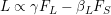
Most of the spread among models in the shortwave feedback is undoubtedly due to clouds, but there is a non-cloud related background positive shortwave feedback –partly due to surface (snow and ice) albedo feedback and partly due to positive short wave water vapor feedback. The latter does not get mentioned much because it is often lumped together with the larger infrared feedback, but it accounts for something like 15% of the total water vapor feedback (water vapor absorbs solar radiation, reducing the amount of solar radiation reaching the surface, so more vapor mean means less reflection from the surface and less loss of energy to space through this reflection.) The surface albedo and water vapor shortwave feedbacks are probably enough in themselves to compete with $\gamma$ . In ESM2M negative short wave cloud feedbacks bring the magnitude of $\beta_S$ down and $\gamma$ is relatively large, resulting in the intuitive response — the outgoing longwave decreasing with time with increasing CO₂.

(The following paragraph corrected on June 1, 2014.) Although it is not directly relevant to the simulations described above, it is interesting to consider the special case in which there is some positive solar forcing added to the positive longwave forcing. For simplicity, let’s just assume that there is no shortwave feedback, so $S = F_S$ (we still have long wave feedback of course). The temperatures will increase if $F_L + F_S$ is positive, and this warming must be due to positive $L + S$ in our simple model (assuming once again that we are in the intermediate regime). But is it $L$ or $S$ that looks like it is causing the warming? A manipulation similar to that above shows that $L \propto \gamma F_L - \beta_L F_S$ .So if the shortwave forcing is larger than $\gamma/\beta_L$ times the longwave forcing — this ratio is something like 25% in the main group of models that we looked at above — the system is being heated by the shortwave rather than the longwave flux even though the shortwave forcing might be much smaller than the longwave forcing.

I guess the moral here, if there is one, is that it is useful to have an explicit model in mind, however simple, when thinking about the Earth’s energy balance and its relationship with surface temperature.

[The views expressed on this blog are in no sense official positions of the Geophysical Fluid Dynamics Laboratory, the National Oceanic and Atmospheric Administration, or the Department of Commerce.]

8 thoughts on “46. How can outgoing longwave flux increase as CO2 increases?”

Fred Moolten says:

June 3, 2014 at 9:01 am

Isaac – That’s quite interesting. What happens, with either the “intuitive” or “counterintuitive” models, if after CO2 quadruples at 140 years, it stops rising and the models are allowed to run to radiative equilibrium? What will the equilibrium OLR, albedo, and temperature change (climate sensitivity) look like compared with what happens if CO2 is instantaneously quadrupled, dropping OLR by about 7 W/m2? Do you have any thoughts about which simulations are more realistic in either the short or long term? Does the historical record offer any clues?
1. Isaac Held says:
  
  June 3, 2014 at 12:14 pm
  
  Fred, those are all interesting questions. I expect a run with instantaneous 4X CO2 to take on the character of the corresponding 1% run but it will take a while to build up the temperature change needed to potentially reverse the sign of the infrared perturbation. It should end up in about the same place in year 140 as the 1% run. As the model equilibrates when holding the CO2 fixed beyond year 140, the heat uptake efficiency drops to zero (the concept is not that useful in this limit) so if the same shortwave feedbacks operate as in the transient run the increase in outgoing OLR should end up even larger than in the 1% runs (but these feedbacks would presumably change somewhat). Someone who has actually looked at these things may need to correct me. As far as comparing to observations, it’s hard because of the short TOA flux records and the associated importance of internal variability and minor forcings. But L+S is constrained by the dynamics in ways that L and S separately are not, so maybe looking in the orthogonal direction (ie at L-S) might suggest something.
Tim Andrews says:

June 4, 2014 at 9:22 am

Dear Isaac,

This is an interesting perspective on the evolution of radiative fluxes in a transient scenario. As an extension to the post, I thought it might be interesting to explore what might happen to OLR if we subsequently reversed the CO2 scenario, i.e. 1%CO2 ramp-up, followed by a 1%CO2 ramp-down. I suppose this could be considered a hypothetical mitigation scenario. Mark Ringer and I used HadGEM2-ES to partly look at this in a recent paper (Andrews and Ringer, 2014 for an open-access pre-print, apologies for the different notation). We too observed that the OLR increased during the CO2 ramp up, but we were then surprised to find that it remained largely unchanged during the ramp-down (i.e. it plateaued), see Figure 1d and Figure 4 (actually we have plotted LW clear-sky, positive downward, rather than OLR).

Your post inspired us to go back and look at this with the simple model to better understand what is going on. On the ramp up, the parameters of the simple model applied to HadGEM2-ES are: gamma ~ 0.5 Wm-2 K-1, beta_sw ~ -0.9 Wm-2 K-1. So the SW feedbacks are larger in magnitude than the ocean heat uptake efficiency and hence the LW flux to space reduces, as you have nicely discussed. On the return ramp-down, a simple linear model is also a good approximation, but only after a decade or so of curvature that comes about due to heat uptake affecting the evolution of the SST patterns, particularly in the East tropical pacific and Southern Ocean (which continue to warm for a decade or so despite the reversal in radiative forcing and global dT). The feedback parameters on the ramp-down are unchanged, but the climate resistance (rho=gamma+beta=F/dT) is larger. In other words, the forcing is symmetric about year 140 but surface temperatures do not come down as fast as they go up (rho ~1.2 Wm-2 k-1 on the ramp up, compared to ~1.6 Wm-2 K-1 on the ramp-down). So one way of interpreting this is that the ocean heat uptake efficiency, gamma, has changed, presumably due to the response of the deep-ocean. Perhaps surprisingly, gamma just so happens to be ~0.9 Wm-2 K-1 on the ramp down in our model, exactly the same in magnitude as the SW feedback parameter. Hence, the LW fluxes do not change despite large changes in CO2 concentration and surface temperatures. Another counterintuitive result perhaps?

Best wishes,
Tim
1. Isaac Held says:
  
  June 4, 2014 at 12:37 pm
  
  Tim, thanks for the reference. I’ll have to think more about the asymmetry in the TOA fluxes between the increasing and decreasing CO2 legs in your run after reading your paper. This seems like a nice standard case to probe how the simple picture in which everything is proportional to forcing breaks down in different models.
2. Nic Lewis says:
  
  June 5, 2014 at 9:34 am
  
  Dear Tim, likewise thanks for the reference to your very interesting paper. I’ve only had a quick read of it as yet, but I have emulated your results by fitting a simple global 2-box model to them. I can obtain a pretty accurate fit for the whole 280 year period: a diffusion-upwelling model might give an even better fit. This seems to indicate that everything is remarkably linear and symmetrical overall between the ramp-up and ramp-down, notwithstanding the asymmetrical behaviour of individual TOA fluxes in HadGEM2-ES. There doesn’t seem to be any evidence of time-varying global climate sensitivity. The same model parameters suit both ramp-up and ramp-down.
  
  The asymmetry in global dT behaviour matches what would be expected as a result of the ocean below the mixed layer (ML) having warmed. One way of looking at this in the 2-box context is that there is ‘warming-in-the-pipeline’ of ~3.6 K after 140 years, of which ~1.4 K becomes realized during the next 140 years, however forcing evolves over that period. Since the down-ramp induces an equal and opposite transient response to the up-ramp, the surface temperature at year 280 just equals that part of the ‘warming-in-the-pipeline’ at year 140 that is realized during the down-ramp.
  
  Whilst heat uptake ‘efficiency’ γ is a useful concept for periods of a few decades, IMO it is not well suited for multidecadal periods over which the non-conservation of energy implicit in the concept leads to increasingly material inaccuracies, particularly when the time-evolution of forcing changes.
  
  I was surprised how well a linear 2-box model emulated HadGEM2-ES’s 1% p.a. CO2 change behaviour, in view of that model’s non-linear early behaviour shown in Figure 1 of Andrews, Gregory, Webb and Taylor (2012) in an abrupt 4x CO2 experiment (the first point is well away from the regression line). May I ask what thoughts you have on this difference in early behaviour? I don’t see why the forcing-adjustment vs feedback issue would cause non-linearity.
  
  FYI, I obtained the best 2-box fit to your results using an ERF for doubled CO2 of 3.2 Wm-2, in between the fixed SST ERF of 3.5 Wm-2 and the regression-based ERF of 2.9 Wm-2, with time constants of 9.32 and 386.3 years and response coefficients of 0.8188 K and 0.6156 K for boxes 1 and 2 respectively. With non-ocean heat sinks ignored, the corresponding effective ML and thermocline/deep ocean depths are 120 m and 1170 m (over the ocean area only). With an ECS of 4.59 K (and thus a climate feedback parameter 0.70 Wm-2K-1) these parameters produce a TCR of ~2.46 K, and surface temperature and heat uptake values close to those in your paper.
Nic Lewis says:

June 5, 2014 at 9:24 am

Dear Isaac,

Thank you for this interesting post, and indeed for many other excellent posts that I have read before but not commented on.

I knew ESM2M was an unusual model, but I had not appreciated how large the differences in LW and SW behaviour were between it and other models. Your analysis makes sense to me, notwithstanding that I have reservations about the degree of approximation involved in use of heat uptake ‘efficiency’ (Jonathan Gregory’s ‘kappa’ method) over multidecadal timescales.

I will make a separate comment in response to what Tim Andrews has written about HadGEM2-ES.
1. Isaac Held says:
  
  June 5, 2014 at 2:58 pm
  
  Nic, thanks,
  
  i probably do overemphasize the “intermediate” regime with well-defined heat uptake efficiency — it’s of limited utility as you say — but i think it is the right idealization for understanding the qualitative behavior of L and S in these 1% simulations.
Brian Mapes says:

June 7, 2014 at 3:07 pm

This helps me understand much better the counterintuitive, surprising first impression of
“Global warming due to increasing absorbed solar radiation”
Kevin E. Trenberth and John T. Fasullo, DOI: 10.1029/2009GL037527

Their plots in YottaJoules (the integral of the radiative energy imbalance) are numbers so huge that I missed an overall point: The radiative imbalance is so small, so much smaller than the forcing, that the subtle term (beta_S + gamma) can govern the size and even the sign of L, without necessarily implying that beta_S itself is huge or surprisingly large.

Comments are closed.

Share this:

8 thoughts on “46. How can outgoing longwave flux increase as CO2 increases?”