51. The simplest diffusive model of oceanic heat uptake and TCR

Posted on October 17th, 2014 in Isaac Held's Blog

(Sign errors corrected — Oct 31)

Vertical diffusion of heat has often been used as a starting point for thinking about ocean heat uptake associated with forced climate change. I have chosen instead to use simple box models for this purpose in these posts because they are easier to manipulate but also because I don’t feel that the simplest diffusive models bring you much closer to the underlying ocean dynamics. But diffusion does provide a simple way of capturing the qualitative idea that deeper layers of the ocean, and larger heat capacities, become involved more or less continuously as the time scales increase. So let’s take a look at the simplest possible diffusive model for the global mean temperature response. This model is typically embellished with a surface box, representing the ocean mixed layer, as well as by some attempt at capturing advective rather than diffusive transport (ie Hoffert, et al 1980, and Wigley and Schlesinger 1985), but let’s not worry about that. I want to use this model to make a simple point about the value of the concept of the transient climate response (TCR).

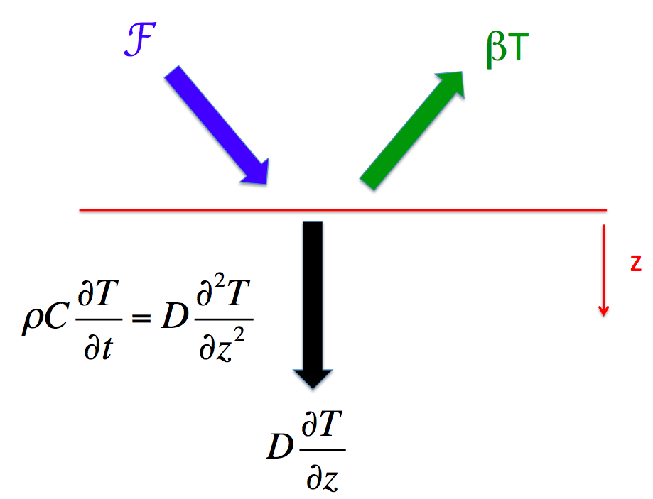
Our equation for the ocean interior is the linear diffusion equation with depth $z$ positive downwards and constant thermal diffusivity $D$

$\rho C \partial T/\partial t = D \, \partial^2 T/\partial z^2$ or $\partial T/\partial t = \mathcal{D} \, \partial^2 T/\partial z^2$

where $C$ is the heat capacity of water per unit mass, $\rho$ the density of water, and $\mathcal{D} \equiv D/(\rho C)$ is a kinematic diffusivity with units of $(length)^2/time$ . The boundary condition at the surface $z = 0$ is

$-D \, \partial T/\partial z = \mathcal{F} - \beta T$

where $\mathcal{F}$ , the radiative forcing, is a prescribed function of time. I am assuming that the ocean is infinitely deep. Fits of this simplest diffusive model to CMIP5 GCM output for idealized forcing scenarios are discussed by Caldeira and Myhrvold 2013.

If we write the boundary condition in terms of the kinematic diffusivity, $-\mathcal{D} \partial T/\partial z = \mathcal{F}/(\rho C) - (\beta/(\rho C)) T$ , the radiative restoring $\beta$ appears in the combination

$\mathcal{V}_\beta \equiv \beta/(\rho C)$

which has units of velocity. Plugging in $\rho =$ 10³ Kg/m³ and $C$ = 4.22 x 10³ J/(Kg K) and, for example, $\beta =$ 2.0W/(m² K), we get 4.74 x 10^-7 m/s for this velocity, or 15 m/year. One way of thinking about this velocity scale is to pick a time scale and compute how deep $\mathcal{V_\beta}$ takes you in this amount of time, which tells you the depth of the layer whose heat capacity gives you a radiative relaxation time for this layer comparable to the time scale that you chose — I think I got that right.] It’s magnitude gives you some feeling for why the oceans are effectively very deep in many climate change contexts.

Together with the kinematic diffusivity we can now define a depth scale $\mathcal{H}$ and a time scale $\mathcal{T}$ :

$\mathcal{H} \equiv \mathcal{D}/\mathcal{V_\beta}; \,\,\, \mathcal{T} \equiv \mathcal{D}/\mathcal{V_\beta}^2$

Climate sensitivity in this simple model is inversely proportional to $\beta$ , which is assumed to be independent of time here for simplicity. So the depth scale $\mathcal{H}$ is directly proportional to climate sensitivity, while the time scale $\mathcal{T}$ is quadratic in the climate sensitivity. This strong dependence of the characteristic time scale on climate sensitivity, with the response of high sensitivity models much slower than in low sensitivity models, is a much commented on feature of this diffusive model. A typical value of the kinematic diffusivity obtained from fits to GCMs is around 5 x 10^-5 m²/s, giving a time scale $\mathcal{T}$ of about 7 years for $\beta$ = 2 and about 28 years for $\beta$ =1.

Defining non-dimensional depth $\zeta = z/\mathcal{H}$ and time $\tau = t/\mathcal{T}$ , we get for the response to a step increase in forcing, $h(\zeta, \tau)$ :

$\partial h/\partial \tau = \, \partial^2 h/\partial \zeta^2$

with the initial condition $h(\zeta, 0) = 0$ and the boundary condition at $\zeta = 0$

$-\partial h/\partial \zeta = 1 - h$ .

Once you non-dimensionalize in this way there are no parameters in the problem at all and you only need to solve the equation once. As in the previous post the response to a spike in forcing is then $g = \partial h/\partial \tau$ and the response to a arbitrary time-dependence in $\mathcal{F}$ is

$T(\tau) = T(t/\mathcal{T})= \int_0^\tau \mathcal{F}(\xi) g(\tau-\xi) d\xi$

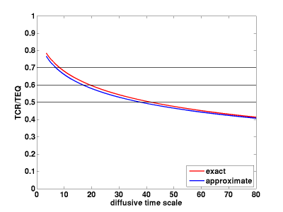
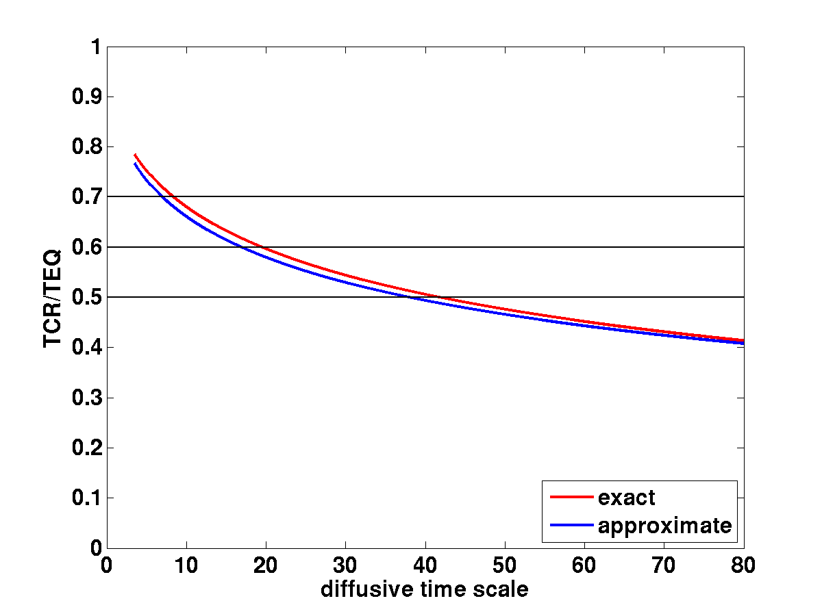
The step-response function $h(\tau)$ is shown below. (I generated this pretty quickly so don’t use it for anything important without checking). Also shown in the figure is a rough approximation to $h(\tau)$ that gets better for large times

$h(\tau) \approx 1/(1 + (\pi \tau)^{-1/2})$

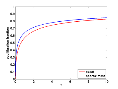
Since the heat uptake by the diffusion is $1-h$ , the heat uptake efficiency (heat uptake per unit temperature) in this approximation is $(\pi \tau)^{-1/2}$ — or, returning to the dimensional form, $\gamma(t) = \beta \sqrt{\mathcal{T}/\pi t}$ — decreasing like $1/\sqrt{t}$ with increasing time. You can use this approximation for $h$ , the response to a step function in forcing, to estimate the response for arbitrary forcing evolution.

Assuming that the forcing is linearly increasing in time, we can compute the fraction of the equilibrium response that is realized at $t = 70 yrs$ , as a function of $\mathcal{T}$ — which we can equate to the TCR . (Increasing CO₂ at 1% per year until doubling, which takes 70 years, is the standard way of defining TCR, and since the radiative forcing is logarithmic in CO2, this implies a linearly increasing forcing. In the context of the linear models being discussed here, the magnitude of the linear trend in forcing is irrelevant;l it is only the time scale of 70 years that is important, as well as the linear shape.) For example, $\mathcal{T} = 20 yrs$ corresponds to TCR/TEQ of about 60%. I have also shown a fit of the following form (which is impressively accurate)

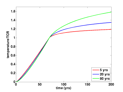
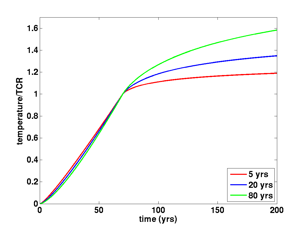
TCR/TEQ $\approx 1/(1 + 1.35 \sqrt{\mathcal{T}/70yrs}) = 1/(1 +1.35 \sqrt{\mathcal{D}/70yrs}/V_\beta)$ .

Here’s a plot of results for a scenario in which the forcing increases linearly for 70 years and then stabilizes, for values of $\mathcal{T}$ = 5, 20, 80 years, but normalized so that they all have the same temperature at year 70, ie the same TCR. It is interesting how tightly the different curves cluster during the growth stage when normalized in this way, separating as one would expect only after the forcing has stabilized.

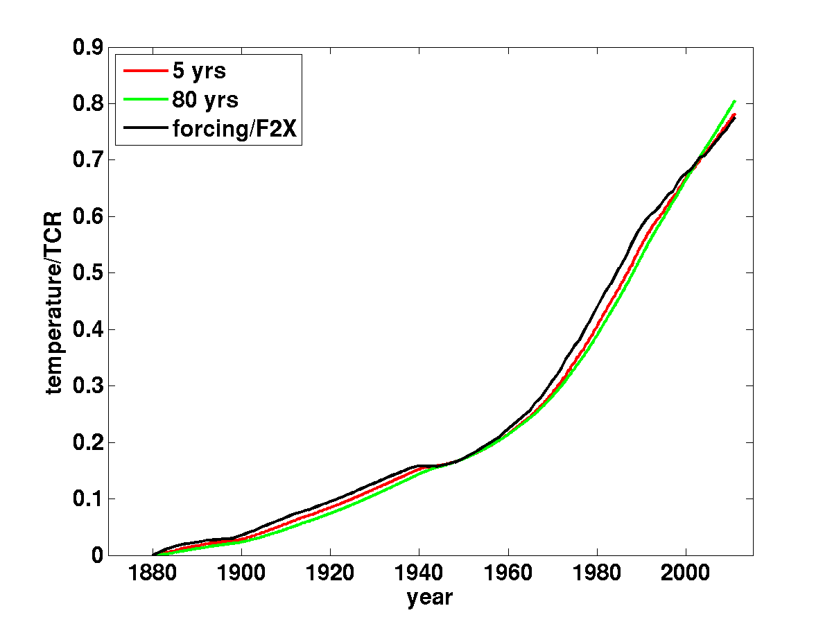
Given the TCR for a particular choice of parameters in this diffusive model, we can also compute the response to the forcing due to well-mixed greenhouse gases (WMGGs) over the past 100 or so years. Does the warming due to the WMGG forcing, which increases monotonically but is far from linear, scale accurately with the TCR? The answer is yes. To see this I have divided the response to WMGGs by the TCR for different values of $\mathcal{T}$ , and plotted them below. (I have used the GISS WMGG forcing. (For this purpose is it just the shape as a function of time that is relevant, not the amplitude.)

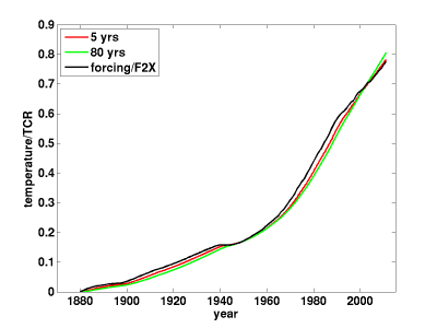
These are identical for most practical purposes, despite the large differences in the diffusive time scale controlling the degree of disequilibrium. I haven’t plotted the case with $\mathcal{T} = 20 yrs$ since that line would have to squeeze between the red and green lines and would be invisible. The claim supported by this plot is that we can confidently use the TCR to predict a model’s response over the 20th century to WMGG forcing. The concept of TCR is sometimes thought of as rather academic since there is no close analog of linearly increasing forcing for 70 years in reality. But in fact TCR provides us with precisely what we want when we try to attribute observed warming to increases in WMGGs. This identification is robust to large changes in heat uptake efficiency. Analyses of GCMs give the same result — see post #3, A statement about the likely range of TCR is equivalent to a statement about the likely size of the forced response to the well-mixed greenhouse gases, or to CO₂ in isolation. This is the main reason that TCR is such a a useful quantity to focus on.

[The views expressed on this blog are in no sense official positions of the Geophysical Fluid Dynamics Laboratory, the National Oceanic and Atmospheric Administration, or the Department of Commerce.]

2 thoughts on “51. The simplest diffusive model of oceanic heat uptake and TCR”

Frank says:

November 10, 2014 at 12:22 pm

Isaac: Intuitively, an practical indicator of diffusion time appears to be the current radiative imbalance to the total radiative imbalance. If diffusion time is 80 years, most of the radiative imbalance built up over the last 75 years should still be present. If diffusion time is 5 years, very little should be relatively little imbalance left.
1. Isaac Held says:
  
  November 10, 2014 at 4:31 pm
  
  Yes, and I think the plot of TCR/TEQ as a function of diffusivity is essentially what you are referring to. Since $\beta$ is assumed constant here, (TEQ-TCR)/TEQ is the ratio of the current imbalance to the total radiative forcing (for the 1% per year run but also a good approximation for the historical WMGG forcing.) I use this large range of time scales just to illustrate how strongly constrained the temperature response is, in the period of increasing forcing, by the value of the TCR.

Comments are closed.

Share this:

2 thoughts on “51. The simplest diffusive model of oceanic heat uptake and TCR”