

Posted on December 19th, 2014 in Isaac Held's Blog
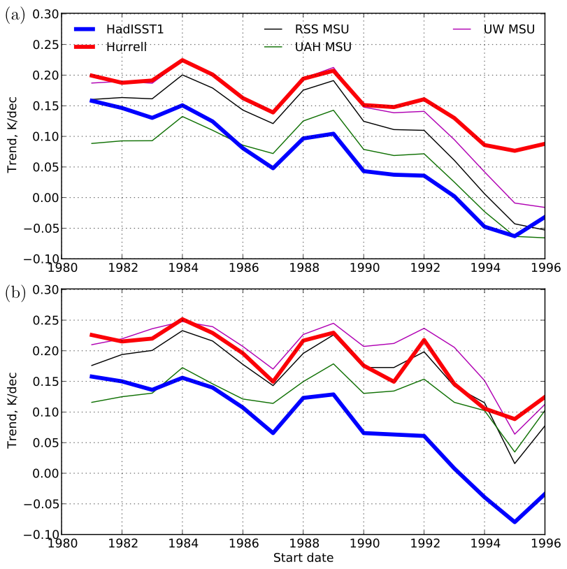 Mid-tropospheric temperature trends (TTT channel — see below) from a given start date till 2008, plotted as a function of start date, in three analyses of the MSU data (thin lines) and in an atmosphere/land model running over two estimates of observed sea surface temperatures: HadISST1 (blue), Hurrell (red). The upper panel is the trend from ordinary least squares while the lower panel uses the Theil-Sen estimator.
In a paper just published, Flannaghan et al 2014, my colleagues (Tom Flannaghan, Stephan Fueglistaler, Stephen Po-Chedley, Bruce Wyman, and Ming Zhao) and I have returned to the question of tropical tropospheric warming in models and observations — Microwave Sounding Unit (MSU) observations specifically. This work was motivated in part (in my mind at least) by the material in Post #21, but the results have evolved significantly. All the figures in this post are from the Flannaghan et al paper.
There are important discrepancies between models and observations regarding tropical tropospheric temperature trends. It is informative if we can divide these into two parts, one associated with the sea surface temperature (SST) trends and the other with the vertical structure of the trends in the atmosphere and how these trends are related to the SST trends. The former is associated with issues of climate sensitivity and internal variability; the latter is related to the internal dynamics of the atmosphere, especially the extent to which the vertical structure of the temperature profile is controlled by the moist adiabat. A moist adiabatic temperature profile is what you get by raising a parcel which then cools adiabatically due to expansion, with part of this cooling offset by the warming due to the latent heat released when the water vapor in the parcel condenses. The tropical atmosphere is observed to lie close to this profile, as do our models. Models continue to approximately follow this profile as they warm., so they invariably produce larger warming in the upper troposphere than at the surface in the tropics — simply because the water vapor in the parcel increases with warming, so there is more heating due to condensation as the parcel rises. All models do this, from global models to idealized “cloud resolving” models with much finer resolution — see Post #20 for a discussion of the latter. The same top-heaviness is seen in the tropospheric temperature changes accompanying ENSO variability, which models simulate very well. Why should lower frequency trends behave any differently than the year-to-year variability resulting from ENSO? If models have this wrong it has a lot of implications.
We study the vertical structure part of the problem using atmosphere/land models running over estimates of the observed SSTs as boundary conditions. The appropriateness of this uncoupled setup will be addressed in the following post, but let’s just assume that it’s OK for the moment. There has been other work along these lines. In particular Fu et al 2011 and Po-Chedley and Fu 2012 helped to motivate our paper. The figure at the top shows some of our results. For this plot, following Fu et al, we use the linear combination of the mid-tropospheric (T2 or TMT) and stratospheric (T4 or TLS) MSU channels, TTT = 1.1 T2 – 0.1 T4, that tries to minimize the weight given to the stratosphere (TTT is also referred to as T24). See also Fu et al 2004. Without this modification, T2 has enough weight in the stratosphere that the large cooling trend there compensates for part of the tropospheric warming trend in T2, making it harder to interpret. The stratospheric trend is primarily forced by ozone changes and is not closely coupled dynamically to the tropospheric trend. I don’t see any reason not to use an adjustment of this kind.
The figure at the top shows the TTT trends averaged from 20S-20N from different start years to 2008, plotting the results as a function of the start year, using three versions of the MSU data and two versions of the model results. (These end in 2008 because some of these runs are taken directly from the CMIP5 archive –we really should update them.) The model results are obtained by using the appropriate vertical weighting of the simulated height dependent trends. The upper panel is the least-square linear slope while the bottom panel is the median of the slopes between all possible pairs of data points. The two model results are from the same model (HiRAM — also discussed in this context in Post #21) but using different SST estimates as boundary conditions — HadISST1 and Hurrell 2008 — the latter being a blend of HadISST and the higher resolution NOAA Optimal Interpolation dataset (see also here). . Hurrel is the boundary dataset recommended for the AMIP (prescribed SST and sea ice) simulations in the CMIP5 archive. Our contribution to the archive with the HiRAM model used the HadISST data instead. Why? It was more convenient for continuity with some other runs that were ongoing and we didn’t think that it made a difference. (We weren’t the only group to do this — GISS evidently did the same thing.) We eventually got around to doing the same simulations with Hurrell and saw the big differences shown in the plot. So on the one hand our stubbornness created some confusion (for example in Fu et al 2011 which shows our model and GISS as standing out from other AMIP simulations). I apologize for this confusion. But on the other hand we might not have noticed this sensitivity to the SST dataset if we had not departed from the script originally.
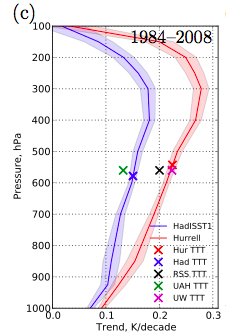
If you look at the tropical mean SST trends themselves they differ in the same sense, with HadISST having smaller trends, but the difference is too small, after accounting for moist adiabatic amplification with height, to explain this tropospheric trend difference. This does not mean that one cannot think of a moist adiabat as connecting the surface air and the upper troposphere, but one has to ask “which moist adiabat?” The upper tropospheric temperature field is quite flat spatially, smoothed out by wave propagation — the appropriate analogy is the flattening of the surface of a pond due to surface gravity waves when you dump a bucket of water in one spot. But the SSTs have a lot of spatial structure in the tropics. Since it is deep convection that couples the surface boundary layer air to the upper troposphere, a natural assumption is that it is the SSTs in the regions of deep convection that matter. Since most of the precipitation in the tropics is related to these deep convective systems, we can think of the precipitation as providing a natural weighting for the importance of the SSTs in different regions. (We are assuming that the relative humidity over the ocean can be thought of a constant here, so the water vapor that is critical for determining which moist adiabat you follow as you rise is itself determined by the temperature.) So we define a precipitation-weighted average of the SST:
where the brackets are an average over the oceans from 20S to 20N. (The rationale for thinking of precipitation over the oceans only in this context will also be discussed in the next post.) Sobel et al 2002 use the same approach when discussing the warming of the tropical troposphere due to ENSO, but in that case the difference between the precipitation-weighted average and straight average is subtle. In the case of trends, this distinction is evidently more important and provides a consistent picture of why the model run over these two different SSTs generates such different upper level trends.
The following figure shows the trends in SSTs (for two different starting years) in different parts of the distribution of tropical SSTs, with the coldest on the left and the warmest on the right. The differences in trend are largest at the warmer end of the distribution of SSTs, which is where the bulk of the precipitation occurs and where the entropy of the boundary layer air is communicated to the rest of the troposphere.
 The three columns of symbols on the left show the unweighted mean SSTs (circles), the SSTs weighted by a time-independent weighting function equal to the climatological precipitation in the model (triangles), and
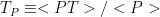
The vertical profiles of the trends in the GCM simulations are shown below, for two different starting dates once again. The shading is the spread of the trends in three realizations of the model with each SST. The smallness of this spread indicates how tightly tropospheric trends in this atmosphere/land model are coupled to the SSTs. The large cooling trends in the model above 100mb are not evident in this plot.
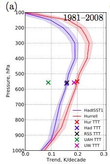
 As in Post #20, to show the estimated MSU trends and the atmospheric trend profiles on the same plot we first compute the levels at which the simulated TTT values obtained from the model — labelled HurTTT and HadTTT — are identical to the actual model temperature trend. These are slightly different between HadISST and Hurrell model runs, so we average them together, and then plot the MSU observations at this level. (If we used the same convention and plotted the unadjusted T2 trends in the same way, this level would be close to the ground!) I like this way of plotting the model profile and the MSU data together — it reminds us that the MSU weighting functions are too broad to catch the actual maximum in the model’s warming trend near 300mb, even though the maximum weight for TTT is near that level. This figure shows pretty vividly how the time period chosen can influence one’s conclusions, as is also evident in the figure at the top. Stephen Po-Chedley obtained very similar results using the Community Atmospheric Model CAM4.
So, if you are trying to make a case for inconsistency between the vertical structure of tropospheric temperature trends in models and observations, you have to pay attention to the SSTs as well as the treatment of the raw MSU data (or radiosondes as the case may be). Not surprisingly, it is the SST trends in the regions of deep convection and precipitation that matter, and this puts more pressure on the quality of the SST data set.
I’ll return in the next post to the question of the legitimacy of decoupling atmosphere and ocean by prescribing SSTs in this way. Can we really use this model setup for quantitative analysis of this kind or is there the potential for significant distortion?
(Special thanks to Stephan Fueglistaler for many conversations on this topic over the past year.)
[The views expressed on this blog are in no sense official positions of the Geophysical Fluid Dynamics Laboratory, the National Oceanic and Atmospheric Administration, or the Department of Commerce.]
The vertical distribution of the observed warming in the tropics is of interest as a test of model fidelity: are observed changes simulated? This new paper is a clear demonstration of the importance of what might seem like subtle aspects of the sea surface temperature trends in affecting the comparison between models and observations.
The vertical structure of the warming is also important for the top-of-atmosphere energy balance (e.g., your posts 24 and 25). Have you and your co-authors examined how this SST-dataset dependence of the simulation results extends to the global-mean energy balance? For example, one might expect the Hurrell-forced simulations to have a bigger trend in OLR, at least for the clear-sky component. This aspect of the simulation results is relevant to Reanalysis-based estimates of climate feedbacks.
Tim,
I did not notice anything as interesting in the TOA energy balance when I looked a while back but I wasn’t thinking about feedback analyses in that context.
Perhaps the next most interesting aspect of these simulations relates to the attribution of trends in Atlantic hurricane frequency.
“Why should lower frequency trends behave any differently than the year-to-year variability resulting from ENSO? If models have this wrong it has a lot of implications.”
In terms of climate sensitivity, what effect would you expect?
I’m thinking of how the GCM spread in precipitation-to-water-vapour increase under warming was 0.09-0.25 in Stephens & Ellis (2008): yet most of the spread in sensitivity was attributed to clouds. Your 2006 paper with Brian Soden and the CMIP5 results reported by Vial et al. show similar things.
Is this relatively tight constraint in the WV/LR feedback helped by the way that models follow the moist adiabat in the tropics?
Mark, I don’t think that it is the moist adiabatic behavior of models in the tropics that limits the effects of water vapor and lapse rate feedbacks on the model spread in climate sensitivity, leaving the spread in cloud feedbacks to dominate. I really prefer the feedback framework formulated in terms of relative humidity rather than humidity itself when thinking about these things — see post #25. This perspective makes clear that as long as relative humidity is more or less fixed you cannot get much feedback from a change in tropical lapse rate. The “lot of implications” that I was referring to had more to do with the adequacy of our models for discussing changes in circulation and precipitation patterns if they are missing this zeroth order behavior of the tropical temperatures.