

FV3: Finite-Volume Cubed-Sphere Dynamical Core
Key Components
Horizontal Discretization
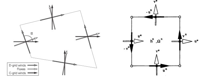
The horizontal discretization of FV3 is essentially the same as the original FV core (Lin and Rood, 1997; Lin 2004), except that all spatial averaging and pressure gradient operators have been upgraded from the 2nd to formally 4thorder accurate in the FV3. The FV shallow-water solver has discretization on D-grid, with C-grid winds which are interpolated from D-grid winds to compute fluxes. For the nonlinear vorticity flux term in the momentum equation, using D-grid allows exact computation of absolute vorticity with no averaging.
More details on the horizontal discretization in FV3 is given in Harris and Lin (2013) and Harris (2016 JCLI, accepted).
The FV Pressure Gradient Computation
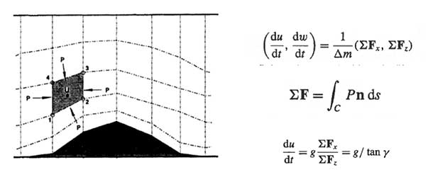
The evaluation of the pressure-gradient force in FV3 remains the same as in the FV core (Lin 1997), upgraded to 4th-order accuracy. A lesser-known aspect of the Lin (1997) algorithm is its consistency with Newton’s 3rd law of motion, achieved by finite-volume integration about a grid cell: the pressure force exerted upon a cell by its neighbor is equal and opposite to that exerted by the cell upon the neighbor. This form satisfies Newton’s third law of motion in the same way fluxform transport schemes satisfy mass conservation. Other algorithms for evaluating the pressure-gradient force do not meet this requirement, with consequences revealed by a simple hydrostatic equilibrium test; see Lin (1997) for details.
A similar test was performed as part of the Dynamical Core Intercomparison Project (Test 200, Ullrich et al 2012): initially resting, hydrostatic atmosphere is imposed upon topography, and the resulting spurious accelerations are then computed. It is found that FV3 produces little spurious oscillation compared to many other schemes.
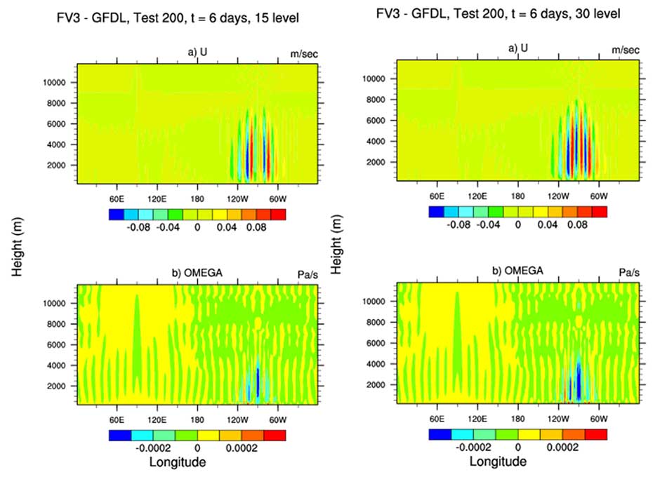
Results at 6 days from DCMIP test case 2-0-0 for two different vertical resolutions.
Vertically Lagrangian Discretization and Non-Hydrostatic Extensions
The Lagrangian vertical coordinate used in FV3 is fully described by Lin (2004). It is a terrain-following pressure coordinate.
Pk=ak+bk*Ps
Equations of motion are vertically integrated to yield a series of layers, and each layer is like a shallow-water system. The 2D horizontal-to-Lagrangian-surface transport and dynamical processes are discretized using the genuinely conservative flux-form semi-Lagrangian algorithm. Time marching is split-explicit, with large time steps for scalar transport, and small fractional steps for the Lagrangian dynamics, which permits the accurate propagation of fast waves.
A mass, momentum, and total energy conserving algorithm is developed for remapping the state variables periodically to an Eulerian terrain-following coordinate to perform vertical transport, and to avoid layers from becoming infinitesimally thin. As long as the layer thickness is positive, the model retains stability. Therefore, there is no vertical courant number limitation in FV3. This is critically important in non-hydrostatic simulations.
FV3 contains two non-hydrostatic solvers for vertical velocity and pressure perturbation. The first, a Riemann solver, was developed at GFDL during 2003-2006 based on a conservative Riemann invariants approach. This algorithm is particularly suitable for ultra-high resolution cloud-resolving simulations, with grid-cell widths of 1 km or less. A variation of this approach, within a simplified 2D vertically-Lagrangian framework, has been published by Chen et al. (2013).
The second non-hydrostatic solver, developed recently for lower horizontal resolutions, is a more traditional semi-implicit time integration scheme for vertically propagating sound waves. This solver is more suitable and more efficient for lower horizontal resolution simulations, in which the extra damping provided by the semi-implicit time-integration scheme can act to filter out the poorly resolved sound waves, and therefore provides a less-noisy simulation. Both solvers use the same governing equations. All FV3 simulations for NGGPS use the semi-implicit solver.
More information about FV3 design and implementation is available at FV3 Documentation and References.