

Posted on October 26th, 2011 in Isaac Held's Blog
Animation of horizontally homogeneous non-rotating radiative-convective equilibrium courtesy of Caroline Muller. The model is SAM (System for Atmospheric Modeling) the principal architect of which is Marat Khairoutdinov. Transparent shading is condensate concentration; colors on the surface indicate near-surface air temperature. See text for further description.
The starting point for most of my thinking regarding climate sensitivity is the simple 1-dimensional radiative-convective model introduced by Suki Manabe and Dick Wetherald in 1967. See also Manabe and Strickler, 1964. For an early review of this kind of modeling, see Ramanathan and Coakley, 1978. Sadly, Dick Wetherald passed away very recently; although it is a very small gesture, I would like to dedicate this post to his memory.
This model solves for a single vertical temperature profile as a function of pressure 


The surface temperature is determined by the net surface radiation and the convective flux at the surface:
Here 

If you integrate such a model to equilibrium without any convective redistribution of energy — ie if you compute pure radiative equilibrium — the result will be strongly gravitationally unstable near the surface. A minimal model of convection might redistribute energy vertically whenever the lapse rate, 


MW don’t actually adjust to the dry adiabatic value. If one does that, the tropopause is too low and the tropospheric lapse rate too large. The observed globally averaged lapse rate is about 6.5K/km. MW simply use this observed value for the critical lapse rate, which results in a reasonable tropopause height. Theories for the observed tropospheric lapse are not easily incorporated in this globally averaged framework, since different mechanisms stabilizing the troposphere are at work in the tropics and in higher latitudes. (In low latitudes, it is more natural to talk about a moist rather than the dry adiabatic lapse rate; in higher latitudes, the large-scale quasi-horizontal turbulence that produces highs and lows and weather competes with smaller scale moist convection in transporting energy upwards.)
In addition, MW do not bother with an explicit diffusive model for the convective transport. Instead they use a simple convective adjustment — while integrating towards equilibrium with a vertically finite-differenced model, check at every time step to see if the flow is unstable according to the prescribed critical lapse rate — if any two layers are unstable set the lapse rate between these two layers equal to the critical value while conserving the mean energy (here this is just the mean temperature) of the two layers. Do this also at the surface to prevent the first atmospheric layer immediately above the surface from being colder than the surface.
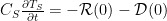
 A figure from Manabe and Wetherald, 1967
The tropopause height is part of the solution. The result for realistic settings is just a troposphere at the critical lapse rate merging continuously at the tropopause into a stratosphere in radiative equilibrium. If you know that this is what the equilibrium looks like, you can get the equilibrium solution by a simpler iteration. For a given surface temperature and tropopause height, the tropospheric temperatures are known. Given these temperatures you can compute radiative equilibrium above this tropopause. The solution will have two problems: the temperature will not be continuous at the tropopause, and the energy flux at the top of the atmosphere will not be zero. These two constraints can then be used to determined the two unknowns — the surface temperature and the tropopause height.
You can do more elaborate things with the surface fluxes and try to simulate the effective air-surface temperature difference, especially if you want to divide the surface convective flux into its two components, evaporation and sensible heat, but this extension doesn’t change the model’s climate sensitivity appreciably.
MW compare the assumption of fixing the relative humidity distribution in the troposphere to that of fixing specific humidities, providing the first modern estimates of the difference this makes for climate sensitivity. Stratospheric water is specified as is the ozone distribution. Clouds must also be prescribed in this model. Increasing the CO2 the surface and troposphere warm by the same amount, by construction, while the stratosphere cools and the tropopause rises, as described in MW. Is this very strong coupling of the troposphere to the surface realistic? I think it is a very good place to start, but my purpose in this post is not to convince you of that but just to convey what this radiative-convective model is.
The strong coupling requires one to think about the energy balance of the surface + troposphere rather than the surface in isolation. Suppose one puts a layer into the troposphere that absorbs some of the solar radiation without increasing the reflection. From a surface energy balance perspective one might guess that this would cool the surface, since less solar radiation would penetrate to the ground. But from the perspective of a strongly coupled surface-troposphere system, whether one absorbs at the surface or in the interior of the troposphere is irrelevant for the temperature response to first order — in fact this absorption would cause warming to the extent that it prevents the scattering to space that would otherwise occur (you maximize this effect by putting the absorber over ice or a low cloud deck.) It is interesting to ask how strong the absorption in the troposphere must be to decrease the convective mixing to the point that the surface decouples from the troposphere. We might call this the “nuclear winter” problem.
In the past one or two decades, there has been an increasing amount of work on radiative-convective models with explicit moist convection. Take your numerical model of the atmosphere and place it over a flat homogeneous surface, ignore rotation, and assume that the geometry is re-entrant in both horizontal dimensions. There are no walls and every point in the horizontal is physically identical to every other point. Assume that the surface is saturated — ie ocean. Turn on the radiative transfer and start destabilizing the atmosphere, evaporating water and generating cumulus convection. Its the same idea as the single column model, but now the model is determining its own clouds and water vapor distribution as well as temperature profile. (Typically one still fixes ozone and stratospheric water). The upper part of the animation above, kindly provided by Caroline Muller, has horizontal resolution of 2km and a square 200 x 200 km domain. This is a statistically steady state achieved after a couple of months of integration. See Tompkins and Craig, 1998 to read more about this kind of simulation. Romps, 2010 is a recent attempt to push to much higher horizontal resolution, to better resolve the key patterns of entrainment and detrainment into and out of the turbulent convective plumes.
The temperature profiles these models produce are qualitatively similar to those generated by single column convective adjustment models, with the moist adiabat determining the critical lapse rate. The surface and troposphere are very strongly coupled in these simulations. I’ll discuss the changes in water vapor and clouds that they simulate in response to CO2 in future posts.
You can get a taste for how these “cloud-resolving models” are compared to data from a variety of observational field programs here. We cannot test them in this homogeneous configuration — you naturally have to simulate the conditions in particular regions in which there have been field programs that provide appropriate data.
The lower panel in the animation at the top of the page is strikingly different from the upper panel, yet it is generated by simply increasing the size of the domain to 512 x 512 km. The convection now aggregates into a small fraction of the domain. See Bretherton et al 2005 for a discussion of this behavior. Caroline and I are currently re-examining theories of this self-aggregation in homogeneous models. The model has hysteresis for some parameter settings, so its climate is not always unique. I find this sort of thing challenging but frustrating as well. We saw something like this in an early low resolution 2-dimensional (x-z) study (Held et al, 1993), but I was hoping that the 3D case would be free of this kind of complexity, so that we could more easily use it as a stepping stone towards understanding more realistic models. Is self-aggregation in the statistically-steady homogeneously-forced non-rotating model a curiosity, or is it telling us something important?
[The views expressed on this blog are in no sense official positions of the Geophysical Fluid Dynamics Laboratory, the National Oceanic and Atmospheric Administration, or the Department of Commerce.]
Sorry I can’t approach this mathematically… anyway:
At least Cb-clouds seem to gather smaller Cu-clouds when they’re growing, I’d imagine the process goes like this: the lowest local air pressure is found under the initial Cb updraft for it is the thickest cloud, this draft creates a slight low pressure between the Cb and surrounding Cu, the clouds merge until there’s enough condensation to counteract the updraft, then Cb is fully matured and the intense downbursts may begin. Whether Cb develops to a rotating supercell would depend on how long the updraft continues to be present (with smaller amount of precipitable water the supercell would be longer-lived (but on this I’m not certain))
The other weather phenomenon where the self-aggregation capability of clouds (I’ve no doubt that it exists, though I’ve got no references) could be of great importance are the oceanic open and closed-cell Sc-clouds in the subtropics, which are always on different locations (one does not find them mixed). This could have an effect to the ITCZ doubling or not as the return flow from the Hadley cell downdraft (the Tradewinds) carry moisture toward the equator.
There are a lot of ways in which moist convection is observed to organize, as you imply, and many of these can be captured in these “cloud resolving” models. But can this organization break the symmetry of the homogeneous system’s climate? In the model generating this animation, the self-aggregation transition only seems to occur in the presence of interactive radiative transfer — if you fix the radiative fluxes it goes away, even though there can still be plenty of clumping and structure in the convection. If you force a vertical shear in the horizontal flow, this phase transition also goes away typically, even though the convection becomes more structured — into propagating squall lines if the conditions are right.
Thanks for this post, and sad news about Dr. Wetherald.
The work in the 1960’s by him and Manabe was pioneering for understanding some of the first-order details of planetary climate (as well as climate change), and the physics outlined here can also serve as the scaffold for interesting thought experiments on Earth as well as on other planets or moons (for example, the strong solar absorption in the upper atmosphere generates an anti-greenhouse effect on Titan, offsetting some of the natural greenhouse effect there).
The work by Manabe and Wetherald is also among the first to synthesize a good enough understanding of spectroscopy and climate physics into a correct conceptual framework for why CO2 warms the planet, following the logic of the top of atmosphere energy balance in the strongly coupled limit, as discussed in your post. Even earlier pioneers such as Plass focused on just the surface budget.
Chris
just to add to the historical perspective, for some reason the work of Hulburt in 1931 is seldom quoted. Though, he recognized the role of convection, of the radiative properties of the upper troposphere and that of ozone in the stratosphere. He also pointed out that it is what he called the radiative region that mainly determines the temperature below and that the radiative properties there are controlled by CO2 more than water vapour.
Maybe it’s true that, in Spencer Weart’s words, climatologists do not read Physical Review 🙂
Riccardo – Thanks for your reference to Hulburt’s work. Can you provide a citation?
Found the abstract here, but the full article is paywalled. It looks like it would be good for instructional (as well as historical) purposes.
Dr. Held: Thanks for this interesting post. How are the boundary conditions at the x-y domain boundaries (in the 3D calculations) specified?
The boundary conditions are doubly-periodic. If there were only one horizontal dimension you could visualize this as the domain being a circle- The last point is identified with the first point. This is a standard setup in statistical mechanics, turbulence theory, etc to create a horizontally homogeneous problem.
Dr. Held,
Thanks for the post. The discussion in the final paragraph of your post is interesting for me because I was thinking about maybe similar things. I recently published a paper on how clouds organize themselves from a statistical point of view: https://www.atmos-chem-phys.net/11/7483/2011/acp-11-7483-2011.html, where my results seem to suggest that aggregation and clumping may be critical to explain the cloud organization we observe from satellite. It would be great to hear about your comments.
The temperature profiles these models produce are qualitatively similar to those generated by single column convective adjustment models, with the moist adiabat determining the critical lapse rate. The surface and troposphere are very strongly coupled in these simulations. I’ll discuss the changes in water vapor and clouds that they simulate in response to CO2 in future posts.
I am really looking forward to that.
I am looking at data from the TAO project: one site at first, then eventually on to all sites. These data record diurnal changes in surface temperature, air temperature, short wave radiation, long wave radiation, relative humidity, wind speed, rainfall and other quantities. Do you think these simulations should be accurately applicable to the column above one of those sites (Pacific Ocean, within 10 degrees N/S of the Equator; there are also some in the Atlantic Ocean and Indian Ocean.)
May I ask another question? Of the heat that is radiatively transmitted to the surface from the sun, and then eventually transferred and radiated away at the top of the atmoshphere, How much is transferred from the lower troposphere to the upper troposphere by radiation, and how much by convection/advection?
Thank you for your time.
These radiative-convective simulations assume that the vertical structure of the atmosphere is determined by the convection (and radiation) that one is simulating within the “column”. For much of the tropics, the local vertical structure is not determined by the local convection and local surface boundary conditions, but by the conditions elsewhere in the tropics where things are more conducive to convection. Atmospheric motions in the tropics are very efficient at communicating the free tropospheric temperature structure determined in the strongly convecting regions to the less active areas. These circulations give you rising motion in regions that are strongly convecting on average and descending motion elsewhere. These vertical motions then strongly modify the water vapor distribution, etc. The radiative-convective model that I describe above has no mean vertical motion.
A way of mimicking local conditions with mean vertical motion is described by Wang and Sobel, 2011, where they relax the model’s temperature structure to a prescribed, tropical mean value. One then computes the vertical motion that is implied by this temperature forcing, and uses this vertical velocity to advect water vapor, etc. You have to do something like if you want to compare a doubly-periodic homogeneous model to the climate in a region in which there is mean upward or downward motion.
As for the magnitude of the convective and radiative exchange between lower and upper troposphere, for a radiative-convective model mimicking the global mean, the convective flux starts out a bit less than 100W/m2 and then decreases with height, providing the warming that stabilizes the troposphere. Radiative cooling just cancels this convective heating, this being due primarily to a net upward longwave flux that increases with height. Most papers on these radiative-convective models seem to provide plots of the heating rates, or vertical flux convergences, rather than the fluxes themselves — ie, Fig. 13 in the Held et al 1993 paper linked to in the post.
Dear Isaac,
Thanks for this interesting description – somehow reminds me of spontaneous symmetry breaking in particle physics. Without knowing any of the relevant literature, I wondered if the fact that in the larger domain case the convection self-aggregates in a region almost as large as the smaller domain size (i.e., 200x200km) means anything. Do you have a feeling for how the size of the convective region depends on the domain size? I.e., if you increased to 1000x1000km, would the single convective region grow or stay at the same size, or would you get two of them? Maybe, the convection’s inherent length scale is 200km (in this particular setup), but if your domain size is just as large as that, convection must be break into smaller individual patches because you need downdrafts somewhere.
And, does the convective region in the large domain size move to a different spot if you wait long enough, or is it sort of fixed in space? In the fist case, you would restore spatial symmetry in the t->infinity limit.; in the second, you wouldn’t for a single simulation.
Aiko,
There are still questions as to the robustness of these results to spatial resolution, something Caroline has some interesting results on. This whole subject remains pretty murky to me.
It seems plausible that, in a model that aggregates, one would get multiple spots if the domain were large enough — I think that happens in some very low resolution hydrostatic simulations using our AM2 column physics — see Held, Zhao, and Wyman, 2007 — in those simulations, a sign of aggregation is that the large-scale takes over from the parameterized convection. Aggregation in that model is favored by increasing SSTs as well. But I don’t have much confidence that those simulations are adequately capturing the dynamics of this cloud-resolving model. One of our goals here is to get something a little closer to ground truth as to what kind of organization is expected in homogeneous non-rotating moist convecting atmospheres, with which to compare the results from models in which GCM column physics is placed in this same homogeneous non-rotating configuration.
I haven’t seen the aggregated convection move appreciably in this configuration, so if the translational symmetry is restored this takes an exceedingly long time.
Isaac,
Could you comment on the sensitivity of the convective self-aggregation to the SST? I was at a seminar recently given by Kerry Emanuel at the University of Albany, who seems to be hypothesizing that the tropics could bifurcate naturally between aggegated and non-aggregated states depending on temperature, or that tropical convection can be in the state of a self-organized criticality.
An implication might be that you could eliminate a source of TC genesis/intensification for example (e.g., by turning off African Easterly waves) but that the tropical ocean-atmosphere system could still adjust to produce a similar number of TC’s on an annual basis. This would seem to have large implications for tropical thermostat mechanisms, and possibly deep-time equable paleoclimates. I was wondering if you had some thoughts on this- it peaked my interest at least, and I suspect some powerful theories could come out of future research.
Chris,
The question of whether self-aggregation in the homogeneous non-rotating model is relevant to tropical storm formation in rotating models is very natural. I will try to write a post on the topic of rotating homogeneous radiative convective equilibrium eventually, a problem that a number of people are working on. But it is a big leap from these homogeneous models to the real world. The idealized configuration can give a very misleading impression as to the dominant controls on things. Right now, I have more confidence in GCM simulations of the statistics of tropical storm genesis, in which we try to push the resolution in a realistic global context, such as those discussed in post #2, than inferences from idealized homogeneous systems. There are some very interesting ideas floating around, admittedly. But I am still not convinced that the self-aggregation described above is not an artifact of the resolution/sub-grid closure in the models.
Hi Isaac,
your site seems to be directed more towards professional climate scientists. So I hope my question is not too naive.
Which behaviour in the two simulations at the top of this page do you commonly find in nature:
self-aggregating or non-self-aggregating?
Cheers,
Martin
Supposedly “naive” questions are often the most important. We see clumping, structure, and organization of different kinds in tropical convection on a wide variety of scales. Whether some of this organization is related to the organization seen in the self-aggregating state of non-rotating radiative-convective equilibrium simulated by some models is an open question. It is not easy to disentangle these things. But I personally do not expect close correspondences between Nature and such an idealized model.
As I have mentioned before on this blog, I try to think in terms of a hierarchy of models of different levels of complexity — some of these models can be useful even if they do not correspond closely to the real world — if they isolate the (possibly unrealistic) dynamics that results from removing other mechanisms at play in reality. Non-rotating radiative-convective equilibrium seems to me to be a very natural element in this hierarchy and a natural step beyond single column radiative-convective models with a simple convective adjustment. Unfortunately we can’t simulate statistically steady moist convective turbulence in the laboratory. I think we are still at the stage of figuring out which aspects of of these computer simulations are robust to the numerics and resolution and which are not.
Hi Isaac. Some things here are of great interest to me, for instance,
“These radiative-convective simulations assume that the vertical structure of the atmosphere is determined by the convection (and radiation) that one is simulating within the “column”.”
Sir, globally, the vertical structure of the troposphere time averaged, is independent of radiation as an influence upon the lapse rate.
dT/dh= -g/Cp, modified by latent heat transfer.
Do you agree or disagree with this comment?
Setting the tropospheric lapse rate equal to a moist adiabat is an approximation that is only useful in the tropics. The extratropical lapse rate is set in a more complex way, with the large scale eddies and small scale convection both doing some of the upward heat flux balancing the radiative cooling. Even in the tropics it is not exact, but in practice it is a good place to start, because convective time scales are much shorter than radiative time scales, so in that sense we are on the same page I think.
Hi Isaac, thanks for the reply. I do not wish to offend in any way, but I cannot understand why the lapse is ‘set’ other than a boundary condition. The lapse should freely evolve from the sum of diabatic processes and the gravitational conditions. It should be possible to switch on a degenerate model (by switching on the Sun) and allow it to evolve from zero altitude at 0K to produce an atmospheric column that reflects reasonably an average section of an atmosphere of a rocky planet, including its average lapse rate and tropospheric height. Both of these are easily calculable from surface temperature and specific humidity. The models physics should produce a reasonable representation of a real world lapse I would hope. Why does it have to be input?
There are, as you probably know, derivations of lapse rates for gaseous envelopes contained by gravity that provide lapse rates similar to those measured on Earth and other planets. These derivations are independent of opacity (ie no reference is made to (internal or ambient) radiation) except from the stand point that Cp ‘already’ includes available vibrational modes that ‘actually’ effect thermal response.
Of course radiation is important as the heating and cooling processes linking the Earth to the Sun and space.
I am confused by this comment. The model pictured in the animations does simulate the tropospheric lapse rate; it is not input into the model. We do impose lapse rates in certain very idealized models of the troposphere. Sorry if it is confusing when I bounce around between very different kinds of models.
There’s an odd set of arguments floating around the web that radiation doesn’t affect the vertical structure of temperature in the troposphere, because you can derive an adiabatic lapse rate without appealing to radiative transfer, and get something close to observed…I never understood it, but perhaps Geoff has found these set of claims. Ultimately radiation is why the troposphere is convecting to begin with, and opacity affects the tropopause height. With a pure N2/O2 atmosphere I’d just expect an isothermal column (has anyone did this?). And radiation is important for the stratospheric temperature inversion.
It’s precisely that the convection helps establish an adiabat so efficiently in the time-mean that for many purposes it’s fine to just prescribe that vertical structure in simple models.
Thanks for the clarification Isaac. I am pleased the the physics employed here is sufficiently robust to produce an authentic lapse rate.
I am really interested in the coupling you have mentioned between the troposphere and the surface. Also, from this, the notion that the surface temperature supported is largely independent of where heat enters the profile. We see strong coupling here on Earth where around 70% of the insolation is thermalised at the surface itself, and strong coupling on Venus virtually no direct solar energy reaches the surface. Yet on both the surface conditions are calculable from the upper troposphere as we can calculate and project an appropriate lapse (surface potential temperature).