

Posted on March 1st, 2012 in Isaac Held's Blog
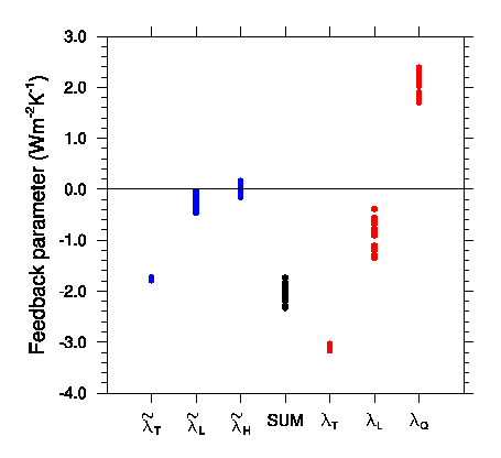 Some feedbacks in AR4 models, from Held and Shell 2012. The three red columns on the right provide the traditional perspective: the “Planck feedback”– the response to uniform warming of surface and troposphere with fixed specific humidity (


This is the continuation of the previous post, describing how we can try to simplify the analysis of climate feedbacks by taking advantage of the arbitrariness in the definition of our reference point, or equivalently, in the choice of variables that we use to describe the climate response. There is nothing fundamentally new here — it is just making explicit the way that many people in the field actually think, myself included. And if you don’t like this reformulation, that’s fine — it’s just an alternative language that you’re free to adopt or reject.
The simplest way to think about this reformulation it that it describes climate change in terms of changes in temperature and relative humidity rather than temperature and specific humidity (or water vapor concentration or vapor pressure). Consistently, the reference response is computed by assuming that the surface and troposphere warm uniformly while relative humidity within the troposphere remains unchanged.
The key is the claim that fixing the relative humidity is a much more natural starting point than fixing specific humidity. I am open to new observations or models that point in a different direction, but I don’t see anything on the horizon that looks like it will modify my personal expectation in this regard. I will try to explain why I feel this way in forthcoming posts. But here are a general comment to think about in the meantime:
We want to use a reference response that is physically meaningful in itself — ie, that doesn’t require “feedbacks” to be present to ensure that it remains physically meaningful as climate changes. But specific humidity can’t remain fixed as we cool the climate — the atmosphere would become supersaturated in a lot of places. And this would happen pretty quickly; the amount of cooling at the peak of the last glacial would be more than enough. Why should fixing specific humidity be a useful starting point as we warm but not as we cool the atmosphere? We would have to argue that there is something special about the position of the present climate in the space of climates with different temperatures.
Using the same notation as in the previous post, and ignoring clouds and surface albedos, in the traditional formulation we have

where the three terms on the right account respectively for the effect on the incoming top-of-atmosphere flux 

where the reference response with fixed specific humidity is 


We now divide 


The decomposition on the left side is shown for the same AR4 models in the blue columns in the figure. Corresponding to this reformulation, we can also define a new reference response, 


So you can describe these model responses as starting with the fixed relative humidity-no lapse rate change reference (about 1.75 (W/m2)/K) with a bit of negative (I had written “positive” originally — IH–3/6) fixed relative humidity-lapse rate feedback (about 0.25 (W/m2)/K) and very small relative humidity feedback, leading to the 2 (W/m2)/K total in the absence of any surface albedo or cloud feedbacks. I think we can agree that this is a simpler picture of the model responses, avoiding the cancellation between the large positive water vapor and negative lapse rate feedbacks.
A key point is that the scatter among the models in the individual terms is now considerably smaller. The tendency for water and lapse rate feedbacks to be negatively correlated across models has been noted since these feedback analyses were first performed across multiple models (Zhang, et al, 1994) and has been discussed recently by Ingram, 2010. (I’ll like to return to Ingram’s paper in a future post — there is also the possibility of going a step further and distinguishing between holding tropospheric relative humidity unchanged at a fixed height and holding it unchanged at a fixed temperature.) At least from this perspective of the model responses, avoiding the negative correlation seems like a very helpful simplification.
Another interesting point is that the fixed relative humidity lapse rate feedback is negative, albeit small. This is the basis for my response to a question on post #20 regarding why I thought that negative lapse rate feedback wins out over increased water vapor feedback when a model’s tropical upper tropospheric warming is increased.
It is also interesting to add other sources of feedbacks, like clouds, into the mix. The cloud feedback as measured by 

It is also worth thinking about this reformulation from the perspective of the issue of skewness in our uncertainty in climate sensitivity (ie Roe and Baker, 2007). If we have a distribution of values of 

Note added March 5:
One e-mail has asked why there isn’t more spread in the “reference” responses, either with fixed specific or with fixed relative humidity. Another e-mail asks why there is any spread at all in these reference responses.
In this paper, we have used a single radiative code for all computations, and we also assume a single unperturbed climate state. We do not use the radiative algorithms or the unperturbed climate states from the individual models. So we are in that sense underestimating the intermodel spread in these reference responses. Differences in clouds in the unperturbed climate states simulated by the models are probably the biggest source of spread (the effects of an increase in temperature or water vapor on infrared emission to space depends especially on what the prescribed high cloud cover is.)
So why is there any spread at all in the 

[The views expressed on this blog are in no sense official positions of the Geophysical Fluid Dynamics Laboratory, the National Oceanic and Atmospheric Administration, or the Department of Commerce.]
Isaac,
I didn’t mean to imply on my comment to the previous post that I don’t like the change. I appreciate your note that the multiplier is 1.77.
Isaac: Your last question is a fascinating one; I am not sure it is a topic well established in the community (I’d love to build up a paper on this), nor do I see this as recognized as a potential issue by Gerard Roe and other key players in emphasizing the relation between uncertainties in and
and  . Here’s what I think are a few key points after some preliminary thinking on the issue, and I’d appreciate feedback (no pun intended) on where I could be thinking about this right or wrong.
1) Suppose we define a parameter that represents the ratio
  , or equivalently,
  =
=  . With respect to uncertainties in feedbacks, we are interested in:
Finally,
The last term on the RHS is essentially zero, since uncertainties in feedbacks should not project onto the no-feedback temperature response. There is a competing effect between the term and the enhanced no-feedback climate sensitivity. We are interested primarily in the uncertainty ratio of the surface temperature response to the feedback factor between your reference system and the traditional Planck-only reference system (that has a multiplicative gain factor
  when used to obtain the full system response),
which is almost certainly less than one, which suggests to me a strong dependence on the interpretation that comes out of the reference system.
2) There is no reason to expect the uncertainty in the strength of the feedback to be symmetric. There is good evidence from paleoclimate, for example, that the “traditional reference system” is supplemented by a feedback factor that is almost certainly greater than ~0.4.
3) This linear analysis breaks down as (in any reference system) gets close to one, since one must consider higher-order terms. Moreover, when
  equals or exceeds one, it does not mean you get a runaway snowball/greenhouse state; this only tells you something about the local structure of the net radiation vs. surface temperature (e.g., a flat or negative relation between OLR and T), and nothing about how that behavior changes as a function of climate. It is a bifurcation that may be a small or large change, but information on the long tail of the climate sensitivity PDF cannot be obtained by plots of
  that let
  get close to one.
I don’t see how anything you say in 1) relates to skewness.
Isaac,
It’s possible I’m misunderstanding your whole point. The direction I went with in your question is whether the Roe and Baker interpretation is an artifact of the chosen reference system, in addition to other criticisms such as their statistical formulation and linearization (e.g., Hannart et al). Clearly the function will be skewed since the slope in a
  plane grows at higher values of
  . The question then becomes at what mean value of
  does the climate currently reside in? If the equilibrium climate sensitivity was 4 C for a doubling of CO2, then your
  is about 0.47, whereas in the traditional analysis it is about 0.7 (due to the weaker term in the numerator). Thus, the interesting question is what the local slope is in a
  plane for a given climate sensitivity in two different reference systems.
I’ve made a plot of this here showing your reference system against the traditional one. The blue line corresponds to some “true” value of climate sensitivity (Note f on the x-axis is ). The two colored rectangles correspond to some interval
  , and the local slope reflects the uncertainty in the temperature response given this uncertainty in the feedback factor.
The point I was emphasizing in my final comment in the post was that exactly the same response, and exactly the same spread in this response, can be the result of very different values of the total strength of the feedback.
Isaac,
I have not been able to access a copy of Ingram 2010 but found the following set of slides from a 2011 presentation which seem likely to cover the same ground:
I found the his Partly-Simpsonian predictor approach fascinating and I think I can see how it relates to what you have laid out here providing that your constant RH temperature kernel differs little from what would remain of the standard clear sky temperature kernel if restricted to exclude the frequency bands dominated by water vapour. It seems to give some additional justification for the new approach and a plausible explanation for the negative correlation in the standard approach.
Hopefully the following will show whether I have understood the concepts.
Expressing the LW radiation flux at TOA as the product of kernels acting on the temperatures and specific humidity (Soden and Held 2006) as follows:
Were the kernels divided into bands determined on whether the frequencies were dominated by water vapour or not we might have:
Then
Rearranging by band:
My understanding of Ingram is that radiation in the water dominated band is relatively independent of temperatures and specific humidity but dependent on the relative humidity. Dividing the equivalent temperature due to specific humidity into two parts to obtain the component due to the change in relative humidity:
giving
Relative independence from temperature for radiation in the water dominated band requires:
or
This can be identified with your (Held and Shell 2012) relative humidity scheme (where the first term being the dependence on relative humidity) provided which is true provided
  making the previous condition
  automatically true. The implication being that the frequency bands dominated by water vapour play little part in you new kernel i.e. a constant relative humidity temperature kernel differs little from what would remain of the standard clear sky temperature kernel if restricted to exclude the frequency bands dominated by water vapour as required by Ingrams.
Setting to regain separate terms for surface temperature and lapse rate temperature difference would give:
which bar the approximation is
If represents the Soden and Held decomposition. By use of two terms
  and
and  one can give the Soden and Held decompostion in terms of the new relative humidity decomposition by adding and subtracting the terms A and B:
Perhaps I understand this or maybe not. Whatever the case I am enjoying your paper and Ingram’s approach.
Many Thanks
Alex
Isaac,
I am confused by the following from Soden et al 2008, where changes in relative humidity are discussed:
“The results are computed by multiplying the shortwave and longwave water vapor kernel by the difference of . The units are also in
  . Positive values indicate regions where the relative humidity has increased as the surface warmed, resulting in an increase in the net upward radiation at the TOA relative to its constant relative humidity value.”
Doesn’t a positive value for correspond to a decrease in RH?
I have noted that the convention regarding the TOA flux seems to be reversed in Fig 5 e.g. “Positive values indicate an increase in net outgoing radiation (i.e., a cooling effect).” when compared to the kernels which could make sense of multiplication by the negation of the change in RH, if that is what it is, but that hasn’t helped my reading of the sentence:
“Positive values indicate regions where the relative humidity has increased as the surface warmed, resulting in an increase in the net upward radiation at the TOA relative to its constant relative humidity value.”
It is the oppositive of what I expected. Both the SW and LW water vapour kernels produce an increase in net incoming radiation with increasing WV so I am missing something, but what?
Please help!
Alex
Alex, corresponds to a reduction in relative humidity. Sorry about that. Thanks for the careful reading. Something about the human mind makes it very hard to catch sign errors while proofreading.
You are right. The caption to Fig.4 should read “Positive values indicate an increase in net incoming radiation (ie a warming effect) …” . And a positive value of