

Posted on June 27th, 2012 in Isaac Held's Blog
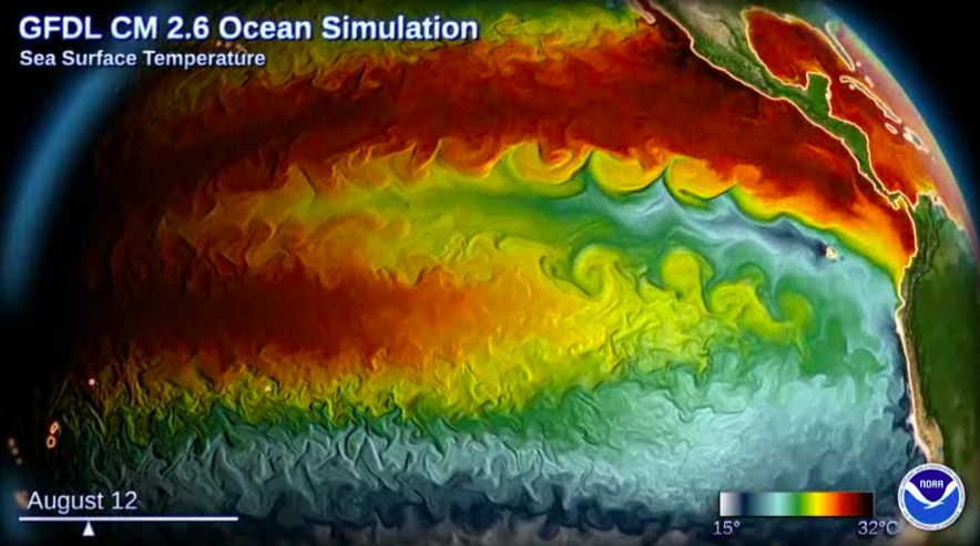
Animation of the sea surface temperature in a coupled climate model under development at GFDL,
the ocean component having an average resolution of roughly 0.1 degree latitude and longitude.
Click HERE for the animation.
(Visualization created by Remik Ziemlinski; model developed by T. Delworth, A. Rosati, K. Dixon, W. Anderson using MOM4 as the oceanic code base.)
As models gradually move to finer spatial resolution we naturally expect to gradually improve our simulations of atmospheric and oceanic flows. But things get especially interesting when one passes thresholds at which new phenomena are simulated that were not present in anything like a realistic form at lower resolution. The animation illustrates what happens after one passes through an important oceanic threshold, allowing mesoscale eddies to form, filling the oceanic interior with what we refer to as geostrophic turbulence. At resolutions too coarse to simulate the formation of these eddies, flows in ocean models tend to be quite laminar except for some relatively large scale instabilities of intense currents of the kind seen in the snapshot north of the equator in the Eastern Pacific. (For a transition comparably fundamental in atmospheric models, one has to turn to the point at which global models begin to resolve the deep convective elements in the tropical atmosphere — see for example Post #19).
When one makes the transition to a mesoscale eddy-resolving ocean model, one is in a sense just catching up with standard-resolution atmospheric models — the eddy production process involved is essentially identical to the process, referred to as baroclinic instability, that generates midlatitude cyclones and anticyclones in the atmosphere. The difference is that the scale at which eddies are generated by this process is much smaller in the ocean than in the atmosphere.
[Theory tells us that a key scale is 


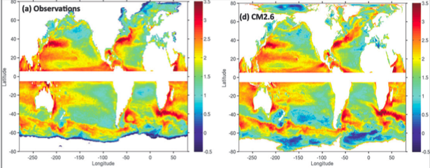
Just as for the high resolution atmospheric simulations animated in posts #1 and #2 , it is a challenge to confront these simulations with observations in the most informative way. One observational constraint that has been especially useful for a first look at the quality of the mesoscale eddy field is the estimate of kinetic energy in the surface flow provided by satellite altimetry. (The horizontal gradient of sea surface height provides an estimate of surface currents through the geostrophic relation.) Here’s a comparison of this model with an observational estimate, described in Delworth et al 2011. Note that the color scale is logarithmic — 
 Among many aspects of these eddy-resolving simulations that are worthy of close study — mesoscale eddies are known to interact with convection in key regions of deep- water formation; eddies and vortices forming around the Cape of Good Hope appear to be important for the saltiness of the Atlantic; and, perhaps most importantly, these eddies help set the strength and structure of the Antarctic Circumpolar Current and its sensitivity to changes in wind and thermal forcing — this being a a key region for heat and carbon uptake. Eddy heat transport across the circumpolar current could play a crucial role in regulating how fast the waters around Antarctica warm. Lower resolution ocean models include closure schemes for the fluxes associated with these mesoscale eddies, but these remain relatively crude (I can say this because I have spent some time trying to develop these theories in both atmospheric and oceanic contexts, as illustrated here.) There is little doubt that direct simulation is better than any existing closure schemes.
On the other hand, these oceanic eddies are not as dominant as they are in the atmosphere. This is at least in part because the basin geometry creates north-south currents that play a significant role in oceanic north-south heat transport, unlike the atmosphere where poleward heat flux is dominated by eddies. (The latitude band of the Drake passage is distinct in this regard, with no meridional coast along which boundary currents can form, making the dynamics in the Circumpolar Current more atmosphere-like. But we’ll have to stay tuned to see how our overall perspective on the role of the oceans in climate change is altered by these eddy resolving ocean models — a problem that is being tackled at a number of modeling centers around the world.
Note: The calendar indicator in the lower left corner of the animation seems to be off.
[The views expressed on this blog are in no sense official positions of the Geophysical Fluid Dynamics Laboratory, the National Oceanic and Atmospheric Administration, or the Department of Commerce.]
Nice to see that this sort of thing has become mainstream. In 1994 I worked with Rainer Bleck and the PSC to use half of their Cray T3D to do an 0.08 degree simulation of the north atlantic using a parallel version of the MICOM model I developed. Like the visualization you linked, this run showed lots of eddy activity and (I’m told) a reasonable gulf stream separation. Of course 2 decades of Moore’s law means you can very nearly do this simulation on a desktop system now.
We run it on GAEA, which is a pretty far cry from a desktop.
True … but you’re running a global coupled ocean/atomosphere model. That 1994 run was using 10GB memory and achieved around 2.4Gflops … you could probably achieve that with a couple of the latest x86 chips, such as the AMD interlagos in GAEA.
Are the well-defined vortex edges visible in any of the thermal satellite or aircraft images like they are in the model video? I am not sure I have seen anything like the 0.1 degree resolution in any SST images.
When I search for images of gulf stream rings– I get things like this, which seem pretty well-defined. It’s entirely possible that model’s of this resolution are missing vortex filamentation processes that would make vortex boundaries look rougher.
I found time lapse videos of SSTs on WUWT’s ocean page (the WUWT reference pages are very useful even if you can’t stand the editorial pages!) from I believe the Navy lab in Monterey, CA – for the Pacific Ocean, they look a lot like your model videos, vortices are quite visible, but with less crisp resolution, as you suggest…
Interesting, this looks almost too detailed if one tries to compare to observations. But if an off topic question is allowed, I read a bit about the spin up of the models and it was stated there that the order of initialization of the processes is important. The question is, is also the order of areal calculations important during the experiments? I’d think as the area of maximum insolation gets most energy, and the energy dissipates to nearby areas, should the variables for this area be calculated first in each cycle? Maybe a stupid question, but one I haven’t seen answered (though I haven’t much seeked for the answer, just read a couple of climate model descriptions (though not read any code)).
All grid points are updated simultaneously every time step in this model (if I understand the question.)
Thank you for the answer, prof. Held.