49. Volcanoes and the Transient Climate Response – Part I

Posted on August 2nd, 2014 in Isaac Held's Blog

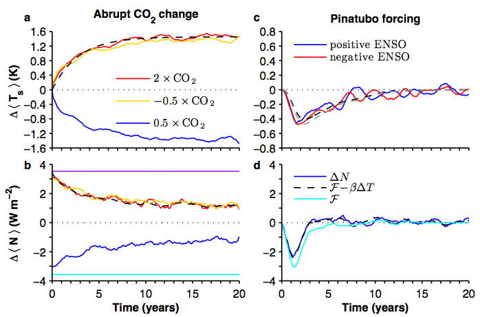Some results on the response of a GCM (GFDL’s CM2.1) to instantaneous doubling or halving of CO₂ (left) and to an estimate of the stratospheric aerosols from the Pinatubo eruption. From Merlis et al 2014.

The following is based on the recent paper by Merlis et al 2014 on inferring the Transient Climate Response (TCR) from the cooling due to the aerosols from a volcanic eruption. The TCR is the warming in global mean surface temperature in a model at the time of doubling of CO₂ when the CO₂ is increasing at 1% per year. You can generally convert the TCR of a model into a good estimate of the model’s warming due to the CO₂ increase from the mid-19th century to the present, or due to all of the well-mixed greenhouse gases, by normalizing the TCR by the appropriate radiative forcing. The TCR of GFDL’s CM2.1 model, one of the two models discussed in Merlis et al, is 1.5K. Can you retrieve this value by looking at the model’s response to Pinatubo? This paper was motivated by the feeling that the literature trying to connect volcanic responses to climate sensitivity has focused too much on equilibrium sensitivity rather than directly constraining the TCR.

Another simulation that has become standard for models is to just double (or quadruple) the CO₂instantaneously and watch the system equilibrate. This gives you more information about the various time scales involved in the equilibration. For CM2.1, the upper left panel shows the evolution over the first 20 years (this is an ensemble mean over 10 realizations with different initial conditions taken from different times in a control run). It also shows a fit with a function of the form:

$T(t) = \mathcal{F}_{2X}\alpha_1 [1 - \exp(-t/\tau_1)]$

with $\mathcal{F}_{2X}$ the radiative forcing due to doubling of CO₂ (3.5 W/m² here — all radiative forcings are computed by holding SSTs fixed, perturbing the system, letting the atmosphere+land equilibrate, and examining the imbalance at the top-of-atmosphere), $\mathcal{F}_{2X} \alpha_1 =$ 1.45K and $\tau_1 =$ 2.8 years. In previous posts, I have discussed how one can interpret this short-time scale response in terms of a simple box model for the surface layers of the ocean,

$c \frac{dT}{dt} = \mathcal{F}(t) -\beta T - \mathcal{H}$

where $\mathcal{F}$ is the radiative forcing, $\beta$ is the strength of the radiative restoring, taking into account all of the radiative feedbacks, and $\mathcal{H}$ is the heat uptake into the deeper layers of the ocean. If we set $\mathcal{H} = \gamma T$ with $\gamma$ the heat uptake efficiency, the heat uptake acts as an additional negative feedback. We then have $\alpha_1 =1/(\beta + \gamma)$ .

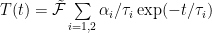
The figure also shows the mean of an ensemble of runs with an instantaneous reduction in CO₂ by a factor of 2. There is a small difference in the ensemble mean, marginally significant at the 10% level, between these warming and cooling switch-on simulations, with $\mathcal{F}_{2X} \alpha_1 \approx$ 1.35K fitting the cooling case. (We checked that the radiative forcing is almost exactly logarithmic in the model, so we can use the same forcing for doubling and halving). This qualitative result might be expected from the picture that cooling at the surface reduces the gravitational stability of the water column, increasing the heat uptake efficiency. But the difference between warming and cooling is small on this time scale, which is nice from the perspective of using a cooling perturbation like a volcanic eruption to infer the transient response to warming.

The model is still taking up heat at about 1 W/m² after 20 years (lower left panel). This model’s equilibrium climate sensitivity is about 3.4K, but it approaches this equilibrium very slowly. Fitting the evolution over longer time scales with a sum of two exponentials,

$T(t) = \mathcal{F}_{2X}[\alpha_1 [1 - \exp(-t/\tau_1)] +\alpha_2 [1 - \exp(-t/\tau_2)]]$

we get something like $\mathcal{F}_{2X} \alpha_2 = 1.9K$ and $\tau_2 \approx$ 400-500 years. This large gap in time scales is clearly the best possible situation if you want to infer a response on the time scale of 50-100 years from the response to a much shorter time-scale forcing. See Geoffroy et al 2013 to place the shape of this response function in the context of that found in other GCMs.

As a first approximation to a volcano, we can set $\mathcal{F}$ to be a spike, a $\delta$ -function, with the result

$T(t) = \tilde{\mathcal{F}} \sum\limits_{i=1,2} \alpha_i/\tau_i \exp(-t/\tau_i)$

where $\tilde{\mathcal{F}}$ is the integral of the volcanic radiative forcing, $\int \mathcal{F} dt$ , which we might call the volcanic radiative impulse. The simple but important point to notice here is the appearance of the factor $1/\tau_i$ . If the magnitudes of the temperature responses to a step increase in forcing on the fast and slow time scales are comparable, the response to impulsive forcing will be much smaller on the long time scale, by the ratio $\tau_1/\tau_2$ . The long weak tail of the volcanic response has been discussed by Wigley et al 2005. Delworth et al 2005 and Gleckler et al 2006 have discussed the closely related long time scale recovery of sea level after a volcano in GCMs. The surface temperature signal on long time scales in the response to a single volcano is effectively unobservable in CM2.1. But given a sequence of volcanoes, the weak long time scale tail would accumulate.

To the extent that one is able to focus on the fast response in isolation we can average over time, returning to the single box interpretation if you like,

$\int_0^{t_0} T(t) dt \approx \frac{1}{\beta +\gamma} \int_0^{t_0} \mathcal F dt = \frac{1}{\beta +\gamma} \tilde{\mathcal{F}} = \alpha_1 \tilde{\mathcal{F}}$

where $t_0$ is a time long compared to the fast decay and short compared to the slow decay. The setup for computing TCR involves linearly increasing radiative forcing (since this forcing is logarithmic in CO₂) for 70 years. For a two-box model mimicking CM2.1, this results in a TCR very accurately given by $\mathcal{F}_{2X} \alpha_1$ . So the estimate of TCR provided by the volcano is

$(\mathcal{F}_{2X}/\tilde{\mathcal{F}}) \int_0^{t_o} T(t)dt$

This integral method does not involve an estimate of the time scale of the fast response.

Merlis et al piggyback on the ensemble of simulations of the response in CM2.1 to the Pinatubo eruption described in Stenchikov et al 2009 which used an ensemble of 20 runs, 10 initialized during an El Nino event in the model’s control simulation and 10 initialized in La Nina events. (Pinatubo occurred during an El Nino, so it is of interest if this modifies the forced response to the volcano. The response is nominally a bit larger in the La Nina ensemble mean, but larger ensembles would be needed to quantify this difference.) The Pinatubo forcing in this model is shown as the light blue line in panel d above. It’s not a $\delta$ -function, but its duration is less than the model’s dominant fast response time. The volcanic radiative impulse is -6.5 Wm^-2-yrs.

The temperature response is shown in panel c. The ensemble mean integrated response up to year 20 is 2.35K-yrs. This gives an estimate of TCR of 1.3K. This is close to the models TCR of 1.5K but a little low. The figure also shows the fit that you get with this one-timescale model, constraining it to fit the integral of the response and using the time scale from the instantaneous doubling simulation. You can also fit the volcanic response varying the two paramaters $\tau_1$ and $\alpha_1$ simultaneously. This two-parameter fit gives an estimate of TCR that is smaller still — about 1.1K. The single time scale model is not a perfect fit to the GCM response.. One can understand the sensitivity to fitting procedure qualitatively if you assume, for example, that the fast response in the GCM actually occurs on two time scales — let’s say 1 year and 4 years, conserving the sum of these two responses and playing with their ratio.

Since the model’s TCR is 1.5K, the underestimate 1.1K is not trivial. It is the sum of little things in this model — the slight difference between warming and cooling perturbations, a small effect in this model of time scales longer than the dominant fast response time, plus a distortion due to the fitting procedure when the fast response itself is not well fit with a single time scale.

We do not need to estimate the separate effects of radiative feedbacks and heat uptake, or $\beta$ and $\gamma$ , to estimate TCR in this way, and there is no need to refer to equilibrium climate sensitivity.

We have used 20 realizations of the response to Pinatubo to get these results. How is this relevant to the problem of determining TCR from a single realization (and without a no-volcano control)? Merlis et al describes what you get if you take one realization of CM2.1, remove the average of the 10 years before the eruption and also remove an estimate of the ENSO contribution based on the relationship between global mean temperature and NINO3.4 SSTs in this GCM. You have to do something like this to get any meaningful results from a single realization, and we don’t claim that this is optimal . We also find it difficult to use the integral method with single realizations, so use the two parameter fitting procedure that results in 1.1K using the ensemble mean response. We get the following:

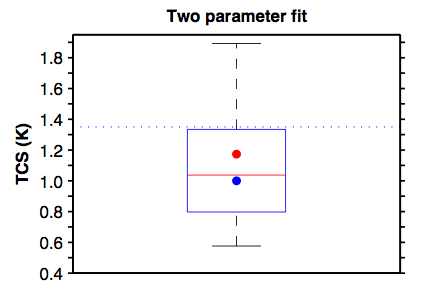The whiskers span the entire range of values obtained from the 20 realizations, the box represents the middle half (25-75%) and the red line the median (with the red and blue dots corresponding to the La Nina and El Nino ensembles). The median is close to the “correct” value of 1.1K for the two-parameter fit. The blue dotted line indicates the value inferred from fitting to the fast response in the 0.5X instantaneous cooling simulation. My suspicion is that this spread is too large, partly because the interanual variability of global mean surface temperature in this model is too big, mostly due to too large an ENSO amplitude — and partly because you can probably do better than this with a better algorithm, possibly multivariate, for isolating the volcanic signal in a single realization. Even with this much uncertainty, this would be useful as one piece of information among others, if coupled to some theoretical guidance for the bias involved.

There’s the rub, I think — because this underestimate could be much larger in reality than in CM2.1 if intermediate time scales play a larger role than they do in this particular model. I’ll return to this issue in Part II.

[The views expressed on this blog are in no sense official positions of the Geophysical Fluid Dynamics Laboratory, the National Oceanic and Atmospheric Administration, or the Department of Commerce.]

10 thoughts on “49. Volcanoes and the Transient Climate Response – Part I”

Fred Moolten says:

August 4, 2014 at 10:29 am

Isaac – In a recent (July 2014) J. Climate paper, Rypdal and Rypdal have suggested that TCR estimates will be affected by the long term memory of previous forcings embodied in disequilibrium between upper and deeper ocean layers – Long term memory effects… implications for future warming. In particular, past negative volcanic forcing would exert a cooling influence on a 1 percent annual CO2 rise, while more recent anthropogenic forcing would nullify this effect and perhaps enhance the TCR rise. As I understand their rationale, they use a power law rather than exponential decay in their model because of the multiple different timescales involved, and report this to give a better fit to data from the instrumental record. What is your take on this approach, and in particular, how important will it be to accurately capture of the effects of the different timescales involved?
1. Isaac Held says:
  
  August 5, 2014 at 8:34 am
  
  Fred,
  Thanks for the heads up on the Rypdal+Rypdal paper. I plan to discuss some of the limitations of the simplest 2-box model in Part II.
Paul_K says:

August 6, 2014 at 11:27 pm

Professor Held,
You might note that fitting a model in time to describe the evolution of ocean heat gain is not necessary for the calculation of the linear feedback term or its inverse, the climate sensitivity per unit forcing. The effective linear feedback can be calculated directly from the integral form of the net flux balance, given that you have available here the time series for net flux, forcing and temperature. From that, the effective climate sensitivity to a doubling of CO2 (i.e. the equilibrium climate sensitivity under the assumption of a linear feedback term) can be calculated directly.
The effective climate sensitivity then of course represents an upper bound on the TCR. Since the governing equation can be integrated from the start of the volcanic radiative impulse (t=0) to any arbitrary time t, it is possible to plot the various estimates of the effective climate sensitivity as a function of time. The small variations represent mostly data errors, since there is negligible model error other than via the assumption that the restorative flux is a simple linear function of temperature. The estimates stabilize fairly quickly.
I have done this on Pinatubo for a number of different observational datasets (net flux, temperature) and forcing estimates; this tends to yield modal estimates of 1.1 to 1.3 degrees for equilibrium climate sensitivity under the assumption of constant linear feedback, subject to choice of dataset.
In addition, I have used a fitted two-body ocean model, (but without making your assumption of invariant deep ocean temperature or infinite-acting ocean), to fit the temperature and net flux data – both directly and in integral form. I get the same range of answers for the effective climate sensitivity, but this allows me to also compute the (lower) TCR for the system.
At first glance, my estimates of effective climate sensitivity seem to be the same as your estimates of TCS, but you appear to be comparing your estimates of TCS directly to TCR (?), rather than as an upper bound on TCR.
My specific concern is that your calculation of TCS is isomorphic with the calculation of an effective climate sensitivity for a single body model, rather than the TCR from a two-body model, and this would explain the similarity of my calculations of effective climate sensitivity and your calculation of TCS. The integral method which I outline above is independent of choice of ocean model and should allow you to test very quickly, if you have not already done so, whether you are calculating an effective climate sensitivity or something different.
Paul_K says:

August 7, 2014 at 9:22 am

Professor Held,

I must correct something I stated in the last paragraph of my post above. Since jotting down the post, I have reexamined some of my solutions in more detail, and note that because of the relatively rapid response time of the matched two-body solution(s), the difference between TCR and effective climate sensitivity is very small – typically less than 6%. Given that this difference is so small, I now doubt whether the calculation of effective climate sensitivity using the integral approach I outlined will offer any discriminatory clarity on the magnitude of error introduced by your modeling assumptions.

I also noted however that, in my two-body solutions, the calculated flux from deep ocean to shallow layer goes through a turning point very quickly (less than 12 months), and the calculated deep ocean temperature goes through a clear minimum in less than 30 months.

These timings will obviously vary depending on the exact partitioning of the shallow and deep heat capacities. However, they do not give me any confidence that the flux from the shallow layer in your model can be captured by your default by assumption to a simple scaling of the surface layer temperature. I do not defend my model on the grounds that it is an accurate reflection of the real world – we know that it is not. However, it does offer a remarkably accurate characterization of the given evolution of net flux, which is all that is required for an accurate estimate of the feedback parameter. And it is able to model equilibration.

For me this reinforces the view that the simplifying assumption of an infinite acting deep layer with invariant temperature is introducing an unnecessary modeling error, the magnitude of which is difficult to estimate. While this assumption may be tolerable (but unnecessary) when considering a multidecadal linear increasing in forcing, the fact that this simplified version cannot model the character of deep flux in the unsimplified version of the governing equation, and the fact that it cannot model an approach to equilibrium sensibly, would seem to make the assumption very unsafe for analyzing the Pinatubo data IMHO.
1. Isaac Held says:
  
  August 7, 2014 at 11:01 am
  
  The “effective climate sensitivity” (ECS) is the 2X forcing divided by $\beta$ , where the latter is estimated from some transient response of interest. (As you know, this is typically an underestimate of a model’s equilibrium climate sensitivity — readers can refer to post #5, for example) As you say, it will be an upper bound to the TCR as estimated from that same transient response, the degree of overestimate depending on the magnitude of the heat uptake. In Merlis et al we tabulate the values of $\beta$ obtained from the top-of-atmosphere flux perturbations in these GCM simulations. Converting to ECS, we get about 2.1-2.2K from the 1%/year or instantaneous doubling simulations, and closer to 1.8K from the Pinatubo simulations. So these are roughly 50% overestimates of the TCR values in each case. (There is no guarantee that the ECS as estimated from Pinatubo would be an overestimate of the TCR from the models 1%/year or historical forcing simulations.) But our goal in this paper was to try to constrain the TCR directly without any information about the TOA fluxes. Also, my primary interest in the simple models is as emulators to help interpret GCM results. GCMs sequester quite a lot of (negative) heat in response to Pinatubo on the 20 year time scale and the simple model needs to reflect that. As I have said elsewhere in these pages, simple emulators can make it easier to critique a GCM — one can argue that the emulator is inconsistent with some observation without having to manipulate the GCM to make the case.
  1. Paul_K says:
    
    August 13, 2014 at 4:20 pm
    
    Professor Held,
    Thank you for your response.
    I recognize that your main purpose was to reconcile parameter estimation via a simple emulator between short term/high frequency and long term/low frequency behavior in the GCM – a noble goal, and one that I wholeheartedly support to improve understanding.
    
    I cannot help feeling however that, if the parameter estimation method is genuinely robust, then we should be able to apply the developed methodology to the observational dataset(s) which the GCM is intended to simulate, as well as being able to extend it to results produced by other GCMs. In this instance, I do not believe that we can.
    
    In fact, the GCM responses, as reported here, seem to present a number of important features which are very different from the available observational datasets, and not just in fine detail.
    One of the key differences is in the relative response timings of the net flux and temperature series. The (60S-60N) temperature low was observed about 14 months after the eruption. The low in TOA net flux from ERBS was observed much earlier – just 3 to 5 months after the eruption. ENSO adjustments do little to change these relative timings of net flux and temperature (Soden et al 2002, Forster and Gregory 2006). This additionally suggests that the early temperature and radiative response is controlled by a shallow surface layer with a heat capacity which is significantly below that of the generally recognized “surface mixed layer” and which therefore translates into a relaxation time measured in months rather than years (Harries and Futyan 2006). The GCM results to which you are matching however show a low in net flux occurring just prior to the temperature low which occurs (in the GCM) somewhere around 18 months after eruption implying a slower response and larger relaxation time.
    
    Secondly, in the observational data, the TOA net flux shows a zero crossover somewhere around 20 months, and stays in positive territory after that. The total heat transfer implied by integrating the negative portion of this curve from eruption to zero crossover seems to be quite tightly constrained to a range 2.0 to 2.7 Watt-years per square meter from the ERBS data. On the other hand, your GCM results show a much larger total heat transfer of around 3.8 Watt-years per square meter, implying a deeper response.
    
    Thirdly, and most importantly of all, your GCM results show an almost negligible positive TOA flux after the “zero crossover”, whereas the ERBS data (or ERBS plus CERES, Wong et al 2005, Loeb et al 2006) show a significant positive flux which starts to repay the energy deficit less than or around two years of the eruption. After 20 years, the net flux in your GCM results seems to be (still) hovering around zero or may even be negative; the temperature is hovering around zero and may even be positive; and yet there still remains a (massive) 2.5 Watt-years-per square meter energy deficit which needs to be repaid if the system is to return to steady-state with no net energy loss from the eruption.
    
    The GCM results (with qualifying adjectives all relative to the observational data) show a slow-responding system which builds a large energy deficit and which is then left with no discerible positive net flux nor temperature differential to repay the energy deficit. As you summarise it: “GCMs sequester quite a lot of (negative) heat in response to Pinatubo on the 20 year time scale and the simple model needs to reflect that.” You are left then with a sort of Maxwell’s Demons argument where you postulate that there must exist a very long term repayment of the deficit via a small but invisible positive net flux driven by a small but equally invisible very long term net negative temperature differential maintained by the missing heat sequestered into the deeper ocean.
    
    Well perhaps so. That may indeed be the only explanation you are left with if your processing of the differenced data from the GCMs is free of assumptive error.
    
    So, while we can obtain a consistent match to the observational data with an (unsimplified) two-body model, which shows shallow (negative) heat invasion and equilibration essentially complete within a 20 year period, the same model cannot be applied to match your GCM results. (I hope that we may agree on this point.)
    
    Your response, I think, is that your emulation is trying to match the GCM results,not the observational data. This still leaves me puzzled. Your methodology relies on the existence of a payback of the energy deficit. Your calculated peak total heat transfer (cooling) in the GCM translates into 3.8 Watt-years/m2; your maximum surface temperature change was about 0.6 degrees. This suggests an “influenced” surface heat capacity of less than 6.3 Watt-years/deg K/m2, which translates into less than 50m of water depth. (We know that this is a gross overestimate since the maximum surface temperature change is achieved with a far lower heat transfer than that obtained at the zero net flux crossover.) How does the GCM manage to cool deep ocean from a shallow fraction of the upper isothermal part of the mixed layer? I don’t think that this can be explained as a local phenomenon given that the aerosol dispersion has a timescale of months.
    
    The TCR of your model from a 1% p.a. experiment is based on a deep heat invasion which is certainly influencing more than the mixed layer. Is it not just possible that the high frequency impulse that you are seeking to model here cannot yield sufficient information to abstract a meaningful estimate of TCR because the high frequency impulse is “seeing” a different ocean?
    My apologies for the length of this post.
    1. Isaac Held says:
      
      August 14, 2014 at 8:54 am
      
      Paul, you raise a lot of interesting points. I hope to take a fresh look at the observations on the response to Pinatubo in the near future, but I tend to take baby steps when approaching an important problem like this. Here I am asking what if we did have good estimates of the volcanic response in surface temperature and of the volcanic radiative forcing, then what do we do with it? More specifically, how would we relate it quantitatively to TCR and the response to WMGGs over the past century. GCMs provide the natural framework for addressing this connection. I am not claiming that the particular model used here is the final answer to this question — more on this in the next post. The emulators help us think about, or just summarize, what the GCMs are doing. It is obviously important if one can make the case that a GCM is totally off base compared to observations of the volcanic response — if that is the case then what is the point of worrying about how the model’s volcanic response is related to its TCR? So I need to return to this (after a short vacation!).
      1. Paul_K says:
        
        August 15, 2014 at 6:35 am
        
        Thank you, Professor Held.
        
        I was not being ironic when I said that I thought it was “a noble goal” to understand and explain the GCM results. Given the reliance placed on the longer term projections from the GCMs, I believe that it is valuable to seek explanation for the volcanic response in (each of) the GCMs, even if it does not match the observational data particularly well.
        
        Please enjoy your vacation. I look forward to your further musings on your return.
        
        I perhaps should have acknowledged a couple of things from your previous response. The first is that I am happy to accept that the short term effective feedback (or effective climate sensitivity) MAY not reflect the longer term ECS. I know from some of your publications that this is something that has puzzled you longer than it has puzzled me. I am sure that I have not caught up with you, but I can (very easily) formulate a linear system which shows curvature in the net flux vs temperature response for a step forcing, but which retains the characteristics of an LTI system – equilibrium temperature varies linearly with magnitude of forcing. I remain agnostic about whether the realworld system does or should display these characteristics, but that is a completely separate conversation.
        Secondly, you mentioned that the ECS (in context, I read “effective climate sensitivity”) derived from the volcano response was “closer to 1.8” deg K. Your tabulated results show feedback values (your β values) of 1.9 and 1.7 for positive and negative ENSO respectively. When combined with your F2x value of 3.52, this yields ECS values of 1.9 and 2.1 respectively – a bit closer to the ECS value from your 2XCO2 experiment than you indicate.
        I went through the process of integrating your data for net flux, temperature and forcing to derive ocean-model-independent estimates of ECS. They are not incompatible with the estimates of 2.1 and 1.9 above, but another curiosity appears. Here are the ECS estimates tabulated for the first 7 years after the eruption:-
        
        Year +ve ENSO -ve ENSO
        1 2.0 2.5
        2 1.5 2.0
        3 1.8 2.1
        4 1.8 2.3
        5 1.7 2.4
        6 1.9 2.2
        7 1.7 2.0
        
        The paper very properly tests and reports the difference in responses from the change in initial conditions prior to and during the eruption, but offers little in the way of explanation. I would be very interested in your thoughts on the matter – but only after your holiday!
        Thanks
        Paul
    2. Isaac Held says:
      
      September 3, 2014 at 6:13 pm
      
      Paul, I can’t address all of your concerns here. I will try to post eventually on comparisons of this model with observations both at the surface and the TOA, from which viewpoint we could then return to some of these issues. We have to be careful not to jump to sharp conclusions based on a single realization from observations, regarding either the surface temperatures or the TOA fluxes. It is an interesting question whether it is easier or harder to isolate the volcanic signal in the TOA (not the forcing itself, but the signature at the TOA of the climatic response to the forcing) as compared to the surface temperature, after removing estimates of internal variability and the effects of other forcings.
      
      As you say, we can hope to get an estimate of the effective climate sensitivity and so an upper bound on the TCR from the TOA fluxes if the strength of the radiative restoring is similar in the volcanic and CO2 ramp up simulations. For CM2.1, they are pretty similar (Table 1 in Merlis et al), but this may not be true in all models so we have to be careful there as well. Merlis et al emphasize working with the surface temperatures in isolation to sidestep this kind of “efficacy” issue and go directly to TCR. We end up with a useful underestimate in this model but it can be a less useful lower bound in other models, as discussed in the next post.
    3. Bill_c says:
      
      September 12, 2014 at 10:22 am
      
      Paul_K,
      
      You say:
      
      You are left then with a sort of Maxwell’s Demons argument where you postulate that there must exist a very long term repayment of the deficit via a small but invisible positive net flux driven by a small but equally invisible very long term net negative temperature differential maintained by the missing heat sequestered into the deeper ocean.
      
      Why? In other words, why force the GCM to be memoryless? What if it returns to a state that conserves energy but at a different internal energy than initial conditions?

Comments are closed.

Share this:

10 thoughts on “49. Volcanoes and the Transient Climate Response – Part I”