

Posted on November 21st, 2015 in Isaac Held's Blog
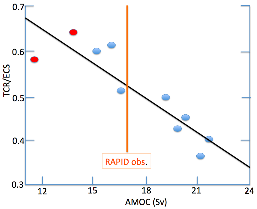
The strength of the Atlantic Meridional Overturning Circulation (AMOC) at 26N , in units of Sverdrups (106 m3/s), plotted against the ratio of the Transient Climate Response to the Equilibrium Climate Sensitivity (TCR/ECS) in a set of coupled atmosphere-ocean climate models developed at GFDL over the past 15 years. Redrawn from Winton et al 2014. Also shown is the strength of the AMOC as observed by the RAPID array at 26N, from McCarthy et al 2015.
An important piece of information about the climate’s response to CO2 (and the other long-lived greenhouse gases) is the degree to which the forced response manages to equilibrate to the CO2 concentration as it increases. Estimates of the degree of disequilibrium affect the attribution of the warming to date as well our ability to anticipate the longer term response to the anthropogenic CO2 pulse. Most of the oceanic heat uptake that determines the degree of disequilibirum occurs either in the Southern Ocean or in the Atlantic Ocean where it is associated with an overturning circulation consisting of less dense waters moving northward near the surface throughout the Atlantic with sinking in the subpolar North Atlantic and a return flow of denser water at depth. I’m focusing here on the latter, the Atlantic Meridional Overturning Circulation, or AMOC. The case for the strength of the AMOC playing an important role in setting the rate of heat uptake by the oceans and the degree of disequilibrium in global mean surface temperature is made in particular by Winton et al 2014 and Kostov et al 2013, who describe two rather different perspectives on why you should expect a relationship between these two quantities.
The Atlantic overturning circulation is difficult to simulate in climate models. Dense waters forming in high northern and southern latitudes compete to fill the deep ocean. The coastal geometry and bathymetry of the sub-polar North Atlantic, where the sinking branch of the AMOC occurs, is complex and often not well-resolved in models used for multi-century simulation. Performing some “geoengineering” of the bathymetry to allow a reasonable pathway for the deep outflow from the Nordic Seas is not uncommon — the dense waters that form need to pass over sharp ridges and through narrow channels. Even if the bathymetry is sufficiently realistic, avoiding too much entrainment of less dense waters into the outflowing dense water (or too little entrainment) is a difficult challenge for ocean models (see Legg, 2009). So we shouldn’t be surprised if climate models produce a range of strengths for the AMOC This is illustrated in the figure above, redrawn from Winton et al 2014, which shows the strength of the Atlantic overturning as measured by the mass flux at 25N in a set of climate models that have been used for research on climate variability and change as well as seasonal-to-decadal prediction at GFDL in recent years. The observational constraint here is from the RAPID array as described by McCarthy et al 2015, whose best estimate for the mean over 2004-2012 is 17.2 Sverdrups. I haven’t put an error bar on this figure (McCarthy et al quote a 0.9 Sv uncertainty for annual means) There is a nominal downward trend in the RAPID data over this time period, and the model results are obtained from pre-industrial control simulations so this is not exactly an apples-to-apples comparison.
Getting a realistic value for the strength of AMOC in a climate model, and it variability, is important for a variety of reasons. (Multi-decadal variability of the AMOC is not robustly simulated across climate models either.) As ocean models move to higher resolution, one would hope that the simulations of the strength of the AMOC and its variability would improve systematically. The red dots in the figure refer to two relatively new models in which the ocean resolution is considerably finer than in the other models. These models are producing relatively weak AMOCs. So this is an ongoing issue (stay tuned — there is a lot of related work underway).
The y-axis in the figure is the ratio TCR/ECS. The Transient Climate Response (TCR) is obtained by looking at the global mean warming at the surface that occurs at the time of doubling when CO2 is increased at 1% /year. The Equilibrium Climate Response (ECS) is the global mean warming after equilibration with a doubling of CO2. The latter is obtained by integrating from a while and then extrapolating carefully. (For those following these things, these are estimates of the models true equilibrium sensitivity, not what is sometimes referred to as the effective climate sensitivity, which is typically smaller. It is also worth keeping in mind that all of these models ignore the responses of the Greenland and Antarctic ice sheets to warming, which would enhance the ECS further if included.) As I have discussed in other posts a model’s TCR is a good guide to how much warming it generates in response to the increase in greenhouse gases from pre-industrial times to the present — you simply need to multiply the TCR by the ratio of the radiative forcing due to all well-mixed greenhouse gases (WMGG) at present to that due to doubling of CO2 (about 0.8). You can then divide this by the ratio of TCR to ECS, to get an estimate of the equilibrium sensitivity consistent with this WMGG-attributed warming. If your estimate of TCR is 1.5K, the implication is that the warming due to the WMGGs up to the present is about 1.5 x 0.8 = 1.2K, (with the implication that aerosol forcing or something else has reduced this to the observed value). A ratio of TCR/ECS of 0.6, say, would give an ECS of 2.5K.
Why would stronger AMOC accompany a smaller ratio of TCR/ECS across models? The argument in Winton et al is less straightforward than you might guess at first. There has been a lot of focus on the possibility of substantial reduction in AMOC strength as the climate warms on decadal-to-century time scales. The Summary for Policymakers of the IPCC WG1/AR5 report assures us that “it is very unlikely that the AMOC will undergo an abrupt transition or collapse in the 21st century for the scenarios considered” ( but is less dismissive of this possibility beyond 2100). However, nearly all models simulate a gradual weakening of the AMOC with warming. Interestingly the AMOC typically recovers eventually as the model climate equilibrates –some models even predict an eventual strengthening, depending in part at least on the competition between the densities in the subpolar North Atlantic and the waters in the Southern Ocean. People have looked at the initial weakening across models and found that the models that have stronger AMOC’s in their control simulations typically have larger reductions in AMOC in 1%/year warming simulations — ie, there is somewhat less spread across the models when you look at the fractional reduction, not too surprisingly.
But AMOC warms the climate on average. You might think that a circulation transporting heat from the southern to northern hemisphere would warm the north and cool the south more or less equally, but because of the asymmetry of the land-ocean configuration, and feedback from northern ice and snow among other things, the northern warming is much larger, resulting in global mean warming with increasing AMOC. (For example, Knight et al 2005 find 0.05K global warming per Sv of AMOC, and 0.09K/Sv in the Northern Hemisphere, in the low frequency variability of their model.) So a decreasing AMOC retards global warming. (As long as the AMOC strength recovers, this retardation is temporary and does not affect the ECS substantially.) Models that have larger AMOCs to begin with simulate larger reduction in this strength with forced global warming, resulting in greater retardation of the warming, providing one perspective on the results in the figure.
A simpler perspective, described in Kostov et al 201 , is that stronger AMOCs are also deeper (think of denser waters formed at the surface in the subpolar N. Atlantic as sinking deeper as well as driving a stronger overturning). So there is a larger effective oceanic heat capacity involved in the heat uptake by this circulation, increasing the disequilibrium in global warming simulations. This argument does not depend on the change in AMOC in response to the warming but just relates to the control models AMOC structure, unlike Winton et al 2014. I encourage interested readers to read these papers and make up their own minds between these two perspectives. But independent of the specifics, it does seem that simulating a realistic AMOC is important for the degree of disequilibrium in model simulations of global warming.
(I had a number of helpful discussions with Mike Winton while writing this.)
[The views expressed on this blog are in no sense official positions of the Geophysical Fluid Dynamics Laboratory, the National Oceanic and Atmospheric Administration, or the Department of Commerce.]
Hi Isaac,
To what extent do you think the Kostov and Winton mechanisms are mutually exclusive? I don’t immediately see why they couldn’t both be operating.
Thanks,
Spencer
Spencer, I don’t see them as being mutually exclusive either. On the other hand, I think that they are separable — for example, by adding some other mechanism to a model that prevented the AMOC from weakening in response to warming.