65. Small Earth, deep atmosphere, and hypohydrostatic models

Posted on December 18th, 2015 in Isaac Held's Blog

A key problem in atmospheric modeling is the large separation in horizontal scales between the circulations that contain the bulk of the kinetic energy and dominate the horizontal transport of heat, momentum, and moisture, and the much smaller convective eddies that provide much of the vertical transport, especially in the tropics.  We talk about the aspect ratio of a flow, the ratio of its characteristic vertical scale to its horizontal scale.  The large-scale eddies dominating the horizontal transport have very small aspect ratios.  These eddies (extratropical storms and even tropical cyclones) are effectively pancakes.  In contrast, the small-scale convective motions have aspect ratios of order one. You have to get the horizontal grid size down well below the vertical scale of the atmosphere — the tropopause height or the scale height — to begin to resolve these small-scale motions. They are not resolved in current global climate models, a fact that colors all of climate modeling. We try to develop theories (closure schemes) for the vertical fluxes by unresolved eddies, but that’s hard and success is limited.  So groups around the world are developing global models with horizontal resolution of a few kilometers.  (The animation in post #19 is produced by a model of this resolution but in a very small domain a few hundred kilometers on a side.)  While these high resolution models don’t resolve all of the vertical transports, global models with horizontal grid size of 1km or so will clearly help a lot.  But we are still pretty far from being able to utilize global models with such high resolution as a flexible tool in climate research.  They are too slow on available computing resources.  So we look for shortcuts.

One important idea consists of embedding a high resolution model into each grid cell of the global model.  The trick is to try to get away with far fewer grid points in each high resolution embedded model than would be needed to cover the whole grid at this resolution.   Often the small scale models are 2D (x and z) rather than 3D (x, y, and z).  The problem is how best to design these small high-res models and how to account for the two-way interactions with the large-scale model.  This multi-grid approach is often referred to as superparameterization.  It is still far more computationally intensive than a typical global climate model.  This multi-scale approach has a lot of promise, but I would like to discuss another, more esoteric, idea here.

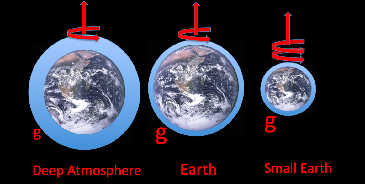
The problem is that the Earth is big.  So why not just make it smaller?  Reducing the planetary radius by a factor of 10, say, would decrease the number of grid points needed to resolve flow with aspect ratio =1  by 100.  Rather than thinking about approaching the desired model by gradually decreasing grid size, maybe we could approach the desired model by gradually increasing the radius of the planet as computational resources allowed, with greater confidence in our simulations of vertical transports at each step along the way.  One obvious problem with this approach is that we don’t have observations of such a planet to compare with our model! In any case the meteorology of such a planet would be very different from our own.  Everything we know about atmospheric dynamics indicates that by reducing the radius by a factor of 10, changing nothing else, we would end up being dominated by an equator-to-pole Hadley circulation.  It would be a totally different atmosphere.  That doesn’t mean that it is entirely without interest, but we can do better.

If we increase the rotation rate by the same factor by which we decrease the radius we are much better off.  One way to see this is to think about a ring of air starting at rest with respect to the surface at the equator, which then conserves its angular momentum as it moves polewards near the tropopause.  If is the rotation rate and is the planetary radius, then it is not hard to show that when it reaches latitude the zonal velocity in the ring will be eastward with respect to the surface, with magnitude .  If we keep the product fixed we end up with the same wind speeds at a given latitude. This flow becomes unstable through a process known as baroclnic instability that depends on this wind speed (actually, the difference between the wind speed near the tropopause and the much slower winds adjacent to the surface). Fixing means that we will have the right kind of instability. For those familiar with baroclinic instability theory, the length scale of the instability will be reduced by a factor of due to the increase in rotation rate, thereby keeping the ratio of this instability scale to the planetary radius unchanged as well.

But now we have another problem.  Even if the wind speeds and eddy scales are ok,  the characteristic time scale of the dynamics, the ratio of the length scale of the eddies (or the planetary radius) to the wind speed, will be reduced.  So the competition between the dynamics and the radiative fluxes and surface frictional effects that controls the circulation will be altered.  But one can try to fix this also by artificially increasing the radiative fluxes and frictional stresses by the factor .  At this point, it feels like we are going down a rabbit hole with no end in sight, but this is the bottom of the hole.  The result is referred to as the DARE approach (diabatic acceleration and rescaling) by Kuang et al 2005.

it is interesting to think about the fruit fly model of post #28 in this context.  This model has the advantage that the radiation and surface friction take the form of linear damping with prescribed time scales.  So in the DARE approach it is unambiguous how to decrease these time scales.  You can then show that the rescaling of radius, rotation rate, and the radiative and frictional relaxation time scales is equivalent to increasing the aspect ratio of the atmosphere.   The large-scale component of the flow remains more or less unaffected because its aspect ratio is so small that it is hardly affected by an increase in this aspect ratio (as long as you don’t use too large a factor ) .

If you actually use the code that produced the figures in post #28 and do this rescaling you find that nothing changes at all!  The resulting model is identical to the model that you start with.  The reason for this is that the model is hydrostatic.  If you have no intention of integrating your model with a grid fine enough to resolve aspect ratio one flows, you might as well drop all terms that are negligible when the aspect ratio is very small.  When you do this systematically, you end up with a hydrostatic model in which the aspect ratio no longer appears in the equations. Nearly all climate models today are hydrostatic. Since the DARE rescaling amounts to increasing the aspect ratio,  this has no effect on hydrostatic models.  Some of us prefer the terminology hypohydrostatic to describe this modeling approach, since you are making the flow less hydrostatic when you increase the aspect ratio of the atmosphere.

Rather than starting out by thinking of making the Earth smaller, we can instead make the atmosphere deeper by reducing the acceleration of gravity, , since the scale height of the atmosphere is inversely proportional to .  The small-scale convection then occurs on a larger scale since the horizontal scale of these convective cells is controlled by their vertical extent.  In the fruit fly model, reducing by the factor , which we might call deep atmosphere rescaling,  is exactly equivalent to and a lot simpler than the DARE rescaling. There is no need to change rotation rate or any damping time scales.   In a hydrostatic fruit fly model, the solution is unaffected by changing .  (To avoid confusion, or maybe create it, in a full hydrostatic GCM changing will affect the solution because this will create unwanted changes in the radiative and frictional damping times, but there are also ways of getting around this.)

Is it useful to approach the desired global nonhydrostatic high-resolution limit by this approach, gradually reducing as computer power allows?  The goal is to improve on the standard models with uncertain closure schemes for the unresolved convective scales.  You can think of this as a kind of convective parameterization.  You distort the convective eddies by making them bigger (think of the deep atmosphere perspective) and then just let the fluid dynamics take over.  I think this question is still open, with some encouraging and some discouraging results to date. See here and here.  If it improves climate models that will be great, but at a minimum I think it helps us to think more clearly about the hydrostatic approximation and which parameters control the shape of the atmospheric circulation.

(Conversations with Steve Garner on this topic have helped me a lot.)

[The views expressed on this blog are in no sense official positions of the Geophysical Fluid Dynamics Laboratory, the National Oceanic and Atmospheric Administration, or the Department of Commerce.]