

Posted on September 11th, 2016 in Isaac Held's Blog
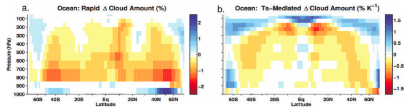
Percent change in zonally-averaged cloud cover over the oceans as a function of latitude and height in response to an instantaneous quadrupling of CO2, decomposed into two parts: (a) a fast adjustment that occurs before surface temperatures have warmed appreciably, and (b) a part that scales linearly with the warming of surface temperature as the system adjusts to the increase in CO2. From Zelinka et al 2013 (as reproduced in Sherwood et al 2015).
The forcing-feedback language used in discussing climate change is familiar but is evolving in interesting directions. I discussed some of the arbitrariness in the decomposition of the feedback into components in posts #24 and #25. (I‘m still serious about discarding the traditional concept of “water vapor feedback” by the way). Here I’ll focus instead on the distinction between forcing and feedback.
In the simplest picture, “forcing” is the result of a radiative transfer calculation that does not depend on the climate response — hold everything else fixed (temperature, water vapor, clouds, etc) and change only the forcing agent (ie CO2); the radiative forcing is the resulting change in flux at the tropopause. But we also speak of “forcing” and “feedback” when emulating GCMs with simple energy balance models. Among other things this helps us isolate the source of differences among GCMs and between GCMs and observations. But these two ideas — forcing as a purely radiative computation, and forcing as a parameter in an emulator of GCM responses — are not fully consistent.
The logic of a “stratospheric adjustment” to forcing has been clear since the work of Manabe and collaborators in the 60’s. Forced stratospheric temperature changes are to first approximation independent of surface/tropospheric changes and adjust to a perturbation in the forcing agent much more rapidly than the latter ( < few months). Their effect on the radiative flux into the troposphere does not scale with the surface temperature change. So it makes sense, especially if interested in time scales long compared to the stratospheric adjustment, to put the consequences of these stratospheric temperature changes on the forcing side of the equation. This has a modest effect for CO2 but it can be more important for other forcing agents, such as ozone.
More recently is has become apparent that fast responses to changes in the CO2 are not confined to the stratosphere in GCMs, but occur in the troposphere as well. Some of these are due to rapid warming of the land surface, but the most interesting are changes in the cloud field over the oceans that occur even when ocean surface temperatures are fixed, due in large part to changes in radiative cooling within the troposphere. See Gregory and Webb 2008. Aerosols produce other complications through their effects on the cloud field, but let’s stick to CO2 for simplicity. Sherwood et al 2015 provide a recent overview of this issue.
When emulating GCMs with simple forcing-feedback models, it’s informative to start with the simplest switch-on simulation: take a control run and increase CO2 instantaneously, then hold it steady and watch the system equilibrate. The figure at the top, from Zelinka et al 2013, shows the change in the cloud distribution over the oceans in an instantaneous quadrupling CO2 simulation, broken up into a fast adjustment and a feedback part. Only the latter part scales linearly with temperature change during the equilibration process. The feedback part in the right panel is the % change in cloud cover per degree K warming; the left hand adjustment part is the % change for 4X increase in CO2. (These are averaged over several GCMs). If the forced warming after 70 years due to the instantaneous 4X increase is 3K say, you multiply the right panel by 3 and add it to the left panel to get the total change. The presumption is that the fast cloud response scales more or less with the traditional radiative forcing, ie, it is proportional to the change in log(CO2). The effect of these cloud changes on the net radiative flux at the top of the atmosphere (TOA) can be split up similarly. (The TOA and tropopause fluxes are basically the same on time scales long compared to the stratospheric adjustment time, but it easier to examine the TOA fluxes to avoid any dependency on exactly how you define the tropopause). There certainly seems to be different physics at play in these two components of the cloud response. The patterns are different over land as well.
The starting point for the simplest energy balance emulator is an expression for the net energy flux at the tropopause N: N = F – βT. Here F is the forcing while β is the net strength of all of the factors restoring the temperature back to equilibrium. N decreases as T, the temperature departure from the control simulation, increases. F is not a function of T but only of the CO2 level. Gregory et al 2004 have advocated for the use of a fit to the N-T relation in the switch-on case (where F is independent of time after the switch on) to define the CO2 forcing F by extrapolating N to T = 0. The key point is to extrapolate using the N-T evolution only after the fast adjustments have played out. (There is some sensitivity to how this is done, hinting that the distinction between adjustments and feedbacks is not totally sharp.) F will then contain the fast tropospheric cloud response and other adjustments. It will not be understandable in terms of a radiative computation in isolation. If you generate a big enough ensemble you can knock down the noise enough to extrapolate all the way back to T=0 and isolate the pure radiative, or instantaneous, forcing, eliminating the stratospheric as well as tropospheric (and land) fast adjustments, but this will not be the best F for fitting the GCM on the longer time scales of interest.
An alternative method for isolating the fast response, utilized systematically by Hansen and colleagues, is to take an atmosphere-land model and then look at the response to an increase in CO2, keeping sea surface temperatures and ice extent fixed. By fixing some things (the slow physics) and letting other things adjust (the fast physics) you are effectively defining what you mean by fast adjustments — the atmosphere and land are fast, the surface ocean and sea ice slow. There can be some differences between these two ways of getting at these fast adjustments, but I won’t try to discuss those here. The left hand panel in the figure above was actually obtained with this alternative approach.
It seems that the cloud response problem has become more complicated, since it now consists of two distinct parts with different physics. You could argue that the fast adjustment is simpler than the feedback component, however. The details of the feedback component can be influenced by the patterns of the ocean surface temperature and sea ice changes which, in turn, involve slower physical mechanisms beyond the relatively fast atmospheric adjustment of the cloud fields once surface conditions are given. This suggests that uncertainty in the fast response might be reduced more quickly as cloud models improve than uncertainty in the feedback component. Maybe we should be grateful that there is a part of the cloud response that is not dependent on the added uncertainties in slow ocean/ice physics.
But can we hope to constrain the fast cloud response to CO2 from observations? I don’t think so — not in any direct way at least . As I have emphasized in a number of previous posts, in GCM responses of the climate response to CO2 over the past century, and that expected over the next century, it is a useful first approximation to assume that N is the heat uptake by the oceans and is proportional to the temperature response T: N= γ T. The implication is that T = F/(β +γ ) so T and F are proportional. This is not valid on the short time scales characterizing volcanic forcing,nor on the long time scales required for the oceans to equilibrate and for N to approach 0. But on intermediate time scales, say 20-100 years, the assumption that forcing and the restoring flux and temperature increase together is supported by GCMs. Now suppose the change in the cloud distribution C can be divided into fast and slow parts as described above, with the fast part proportional to the radiative forcing and the slow part to the temperature perturbation: C = CF + CS = μ F + κ T. But in the intermediate regime, F and T are proportional, so the ratio between the two parts will be unchanged in time (assuming that μ, κ, β, and γ are all constant in time) and observations of trends in clouds will not provide any way of separating the two parts. The bottom line is that we can readily separate these two pieces of the cloud response given an abrupt change in CO2, but we don’t have one of those to study. (And there is no reason to believe that the cloud response to volcanic forcing bears any simple relation to the fast response to a CO2 increase.)
Some final comments:
People have tried to find emergent constraints for cloud feedback — something that is observable and is well-correlated with cloud feedback across model ensembles for clear physical reasons.(e.g Klein and Hall 2015 — see also posts #12 ). Is there value in looking for an emergent constraint for the cloud forcing adjustment in isolation?
The Gregory forcing F (obtained by extrapolating back to T = 0 in a 4X simulation) is substantially anti-correlated with the cloud feedback (e.g. Caldwell et al 2016). Why should that be?
Maybe trying to define two classes of responses — forcing adjustment and feedback — is too fuzzy. The underlying issue is the dependence of the climate response on the time scale of the forcing. Would we be better off testing our emulators against GCM simulations in the frequency domain, with periodic forcing of different frequencies, rather than in the time domain where the different physics at different time scales get superposed — e.g.MacMynowski et al 2011. I am not sure why this is not more popular. One issue may be that this is putting too much weight on the linearity of the response, since we have to go back to the time domain ultimately.
[The views expressed on this blog are in no sense official positions of the Geophysical Fluid Dynamics Laboratory, the National Oceanic and Atmospheric Administration, or the Department of Commerce.]
In this blog post, these changes are called “fast” because of the troposphere timescale that governs them. A potential source of confusion that I’ve encountered is when the term “fast” is used for simulations with prescribed SST: one can simply integrate a model with prescribed SST and perturbed CO2 for a long time (~20 years) to define the fast response. It may cause confusion to define a “fast” change using a 20-year time mean.
In the Sherwood et al. 2015 BAMS paper, the term “adjustment” is used. However, I’d argue that we want to call them “direct” changes. Conceptually, we are separating temperature-dependent responses from those that occur in proportion to the forcing agent change (a Taylor series). We can do this for any variable of interest, such as the cloud amount described here. We can say, beyond the temperature-dependent change in cloud amount, there is a direct response of cloud amount to CO2 or a cloud amount adjustment to CO2. Either of these is clear to me.
Having recognized the generic utility of this type of decomposition, what if we chose to go back to one of the radiation variables that prompted the discovery of these direct changes? If we analyze outgoing longwave radiation (OLR) in this manner, I prefer to say that OLR responds directly to CO2 rather than describing it as an OLR adjustment to CO2… The history of the science and terminology leads to calling the forcing itself an adjustment.
Tim, I think of the 20 year mean using an atmosphere/land only model (if that is the standard convention) as primarily to reduce the noise level — not to include responses that are longer than a a few years. But this is fuzzy in that some parts of the land are slow (permafrost, vegetation, deep soil layers). Do you disable the slow parts? Using the full coupled model is less ambiguous, but the switch on simulation excites all time scales so it’s fuzzy how you to isolate the time scales of interest.
“And there is no reason to believe that the cloud response to volcanic forcing bears any simple relation to the fast response to a CO2 increase.”
Not sure if I understand this post well enough to comment, but I was wondering if a CH4 spike would be similar enough. In that case it might be worthwhile to study that problem so that we know what to measure if that ever occurs.
A methane spike would be close enough I suspect. To get useful information on clouds etc from a single spike, in the presence of internal variability, it would have to be pretty large– not something to wish for.
Issac, why should we pay any attention to transient phenomena that develop during instantaneous 4X experiments? Such phenomena are never going to occur in the real world. I find the whole idea of extrapolating ECS from instantaneous 4X experiments somewhat risky, because the most critical time points (the first 5-10 years) for determining the slope come from a planet under fairly abnormal conditions: a) The fast responses which you discuss above. Some of these may arise from increased radiative cooling by 4XCO2 in the troposphere which dominates the increase in radiative warming (absorption), which would produce a less stable lapse rate and more convection. b) Warming below the mixed layer won’t be able to keep up with warming of the mixed layer, which should decrease vertical convection in the ocean.
Not sure if I understand this post well enough to comment, but I was wondering if a CH4 spike would be similar enough. In that case it might be worthwhile to study that problem so that we know what to measure if that ever occurs.