

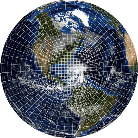
FV3: Finite-Volume Cubed-Sphere Dynamical Core
Quick Links
The GFDL Finite-Volume Cubed-Sphere Dynamical Core (FV3) is a scalable and flexible dynamical core capable of both hydrostatic and non-hydrostatic atmospheric simulations. The design of FV3 was guided by these tenets:
- The discretization should be guided by physical principles as much as possible.
- A fast model can be a good model, but a good model must be a fast model! Computational efficiency is crucial.
FV3 was “reverse engineered” to incorporate properties which have been used in engineering for decades, but only first adopted in atmospheric science by FV3.
FV3 is the dynamical core for all GFDL weather and climate models, including the world-leading AM4 and the powerful SHiELD unified weather-to-subseasonal prediction model and SPEAR seamless coupled prediction system. FV3 has been chosen as the dynamical core for the Unified Forecast System (UFS), formerly the Next Generation Global Prediction System project (NGGPS). The UFS is designed to unify the National Weather Service’s suite of prediction models, including the operational Global Forecast System (GFS) and regional models to run as a unified, fully-coupled system in the NOAA Environmental Modeling System infrastructure. FV3 was successfully implemented within the GFS, and the FV3-based GFSv15 became operational on 12 June 2019. Since then, the GFS and GFS Ensemble have both received further updates to FV3 and other model components. An FV3-based limited area model was implemented operationally in 2019 in the High-Resolution Ensemble Forecast (HREF), and form a key role in the upcoming implementations of the Hurricane Analysis and Forecast System (HAFS) and Rapidly-Refreshing Forecast System (RRFS).
FV3 is also the dynamical core for NASA’s GEOS global model, NASA’s next-generation Mars Climate Model, and for other systems worldwide.
This website describes FV3, including the evolution of its development, basic algorithm, and its global variable resolution capabilities, in both nested and stretched grid configurations. The Performance page explains how efficient FV3 can be.
Dynamics isn’t the whole story. Coupling to physics and the ocean is necessary! Please see the Applications page for the family of models using FV3 and examples of how FV3 has been successfully implemented.
Development History
Finite-Volume Schemes
The FV core started its life at NASA/Goddard Space Flight Center (GSFC) during early and mid-90s as an offline transport model with emphasis on the conservation, accuracy, consistency (tracer to tracer correlation), and efficiency of the transport process. The development and applications of monotonicity-preserving Finite-Volume schemes at GSFC were motivated in part by the need to have a “fix” for the noisy and unphysical negative water vapor and chemical species (Lin et al. 1994, and Lin and Rood 1996). It subsequently has been used by several high-profile Chemistry Transport Models (CTMs), including the NASA-community GMI model (Rotman et al., 2001), GOCART (Chin et al., 2000), and the Harvard University-developed GEOS-Chem model. This transport module has also been used by several climate models, including the ECHAM5 AGCM.
Shallow-Water Model
Motivated by the success of monotonicity-preserving FV schemes in CTM applications, a consistently formulated shallow-water model was developed. This solver was first presented at the 1994 PDE on the Sphere Workshop, and years later published by Lin and Rood (1997). The Lin-Rood algorithm for shallow-water equations maintains mass conservation and a key Mimetic property of “no false vorticity generation”, and for the first time in computational geophysical fluid dynamics, uses high-order monotonic advection consistently for momentum and all other prognostic variables, instead of the inconsistent hybrid finite-difference and finite-volume approach used by practically all other “finite-volume” models today.
FV Hydrostatic Dynamical Core
The full 3D hydrostatic dynamical core, the FV core, was constructed based on the Lin-Rood (1996) transport algorithm and the Lin-Rood shallow-water algorithm (1997). The pressure gradient force is evaluated by the Lin (1997) finite-volume integration method, derived from Green’s integral theorem based directly on first principles, and demonstrated errors an order of magnitude smaller than other well-known pressure-gradient schemes. Finally, the vertical discretization is the “vertically Lagrangian” scheme described by Lin (2004).
From FV to FV3
The most unique aspect of the FV3 is its Lagrangian vertical coordinate, which is computationally efficient as well as more accurate given the same vertical resolution. Recently, a more computationally efficient nonhydrostatic solver is implemented using a traditional semi-implicit approach for treating the vertically propagating sound waves. An experimental vertical Riemann solver option solving for sound waves nearly exactly is under development. A description of the non-hydrostatic extension can be found on the Key Components page.
Moist thermodynamics and variable-resolution FV3
Water is an essential part of the atmosphere’s circulation, but most dynamical cores ignore its effect on heating rates, masses, and other thermodynamics. FV3 has an advanced rigorous implementation of the effect of moisture and water condensates on the dynamics. FV3 also implements a number of powerful capabilities for enhanced resolution, including grid nesting, grid stretching, telescoping nesting, and a limited-area capability for short-range modeling.