November 6th, 2019
Key Findings
- A team at GFDL has developed a new model of the physical climate system referred to as CM4.0.
- Strengths of the model include its ENSO simulation and small biases in TOA fluxes, precipitation, Arctic Sea ice extent, and sea surface temperature.
- Problematic aspects include large variability in the Southern Ocean and a historical simulation with little warming prior to 1990.
I.M. Held, H. Guo, A. Adcroft, J. P. Dunne, L.W. Horowitz, J. Krasting, E. Shevliakova, M. Winton, M. Zhao, M. Bushuk, A.T. Wittenberg, B. Wyman, B. Xiang, R. Zhang, W. Anderson, V. Balaji, L. Donner, K. Dunne, J. Durachta, P. Gauthier, P. Ginoux, J-C. Golaz, S.M. Griffies, R. Hallberg, L. Harris, M. Harrison, W. Hurlin, J. John, P. Lin, S.J. Lin, S. Malyshev, R. Menzel, P.C.D. Milly, Y. Ming, V. Naik, D. Paynter, F. Paulot, V. Ramaswamy, B. Reichl, T. Robinson, A. Rosati, C. Seman, L. Silvers, S. Underwood, N. Zadeh. Journal of Advances in Modeling Earth Systems (JAMES). DOI: 10.1029/2019MS001829
This paper describes the GFDL’s latest multi-purpose atmosphere-ocean coupled climate model, CM4.0. It consists of GFDL’s newest atmosphere and land models at about 100 km horizontal resolution, and ocean and sea ice models at roughly 25 km horizontal resolution. A handful of standard experiments have been conducted with CM4.0 for participation in the Coupled Model Inter-comparison Project Phase 6 (CMIP6), an archive of climate model results utilized by the Intergovernmental Panel on Climate Change (IPCC) and the climate research community more generally.
The model results have been extensively evaluated against observations. This paper makes the case that CM4.0 ranks high among state-of-the-art coupled climate models by many measures of bias in the simulated climatology and in its ability to capture modes of climate variability, such as the El Niño-Southern Oscillation and Madden-Julian Oscillation. The paper also discusses some potential weaknesses, including unrealistically large internal variability in the Southern Ocean and insufficient warming before 1990 in the simulation of the 20th century.
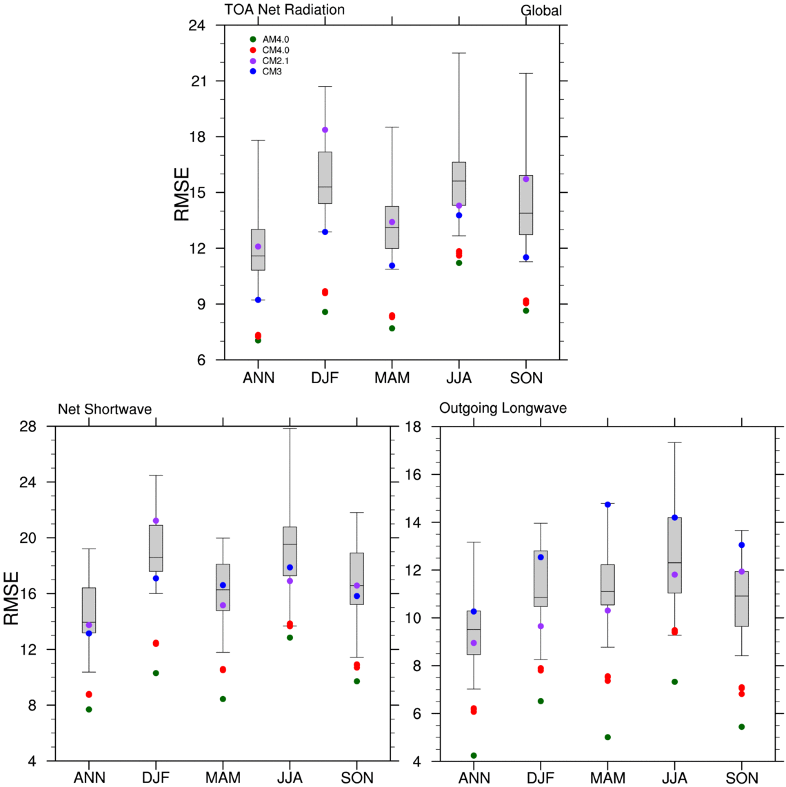
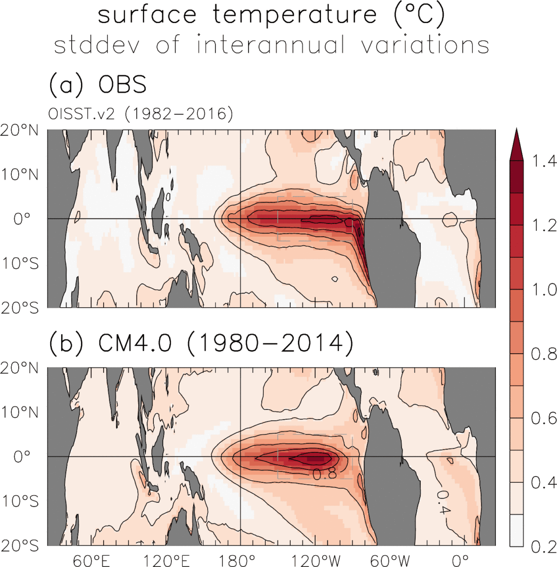
The two figures below illustrate the quality of CM4.0’s simulation of the current climate. The first figure compares the spatial pattern of the top-of-atmosphere (TOA) radiative fluxes with that of the CMIP5 coupled climate models used in the last IPCC assessment. CM4.0 has lower root-mean-square errors in (red dots) than nearly all CMIP5 models (box and whiskers). The second figure shows the realism of the pattern of sea surface temperature anomalies in a typical ENSO event in CM4.0, a marked improvement over other GFDL models used in IPCC assessments (not shown).


