

Posted on June 13th, 2011 in Isaac Held's Blog
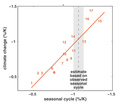 From Hall and Qu, 2006. Each number corresponds to a model in the CMIP3 archive. Vertical axis is a measure of the strength of surface albedo feedback due to snow cover change over the 21st century (surface albedo change divided by change in surface temperature over land in April). Horizontal axis is measure of surface albedo feedback over land in seasonal cycle (April to May changes in albedo divided by change in temperature). The focus is on springtime since this is a period in which albedo feedback tends to be strongest.
There are a lot of uncertainties in how to simulate climate, so, if you ask me, it is self-evident that we need a variety of climate models. The ensembles of models that we consider are often models that different groups around the world have come up with as their best shots at climate simulation. Or they might be “perturbed physics” ensembles in which one starts with a given model and perturbs a set of parameters. The latter provides a much more systematic approach to parametric uncertainty, while the former give us an impression of structural uncertainty— ie, these models often don’t even agree on what the parameters are. The spread of model responses is useful as input into attempts at characterizing uncertainty, but I want to focus here, not on characterizing uncertainty, but on reducing it.
Suppose that we want to predict some aspect P of the forced climate response to increasing CO2 and that we believe a model’s ability to simulate an observable O (let’s think of O as just a single real number) is relevant to evaluating the value of this model for predicting P. For the i’th model in our ensemble, plot the prediction Pi on the y-axis and the simulation Oi on the x-axis. (I am thinking here of averaging over multiple realizations if needed to isolate the forced response.) The figure shows a case in which there is rather good linear relationship between the Pi‘s and Oi‘s. So in this case the simulation of O discriminates between model futures.
Now we bring in the actual value of O — the vertical shaded region in the figure. Because the simulated value of O discriminates between different predicted values of P, the observations potentially provide a way of decreasing our uncertainty in P, possibly rather dramatically, The relationship between O and P need not be linear or univariate, but there has to be some relationship if we are to learn anything constructive about P from the observation of O. And the observed value of O need not lie in the range of model values — if the relationship is simple enough extrapolation might even be warranted. This will all seem obvious if you are used to working with simple models with a few uncertain parameters. But when working with a global climate model, the problem is often finding the appropriate O for the P of interest.
Consider the effects of global warming on Sahel rainfall. This problem grabbed my attention (and that of several of my colleagues) because our CM2.1 climate model predicts very dramatic drying of the Sahel in the late 21st century (see here and here). But this result is an outlier among the world’s climate models. In fact, some models increase rainfall in the Sahel in the future. Using different criteria, one can come to very different conclusions about CM2.1’s relative fitness for this purpose. For example, if one just looks at the evolution of Sahel rainfall over the 20th century, the model looks pretty good (the quality of the simulation is quite stunning if one runs the atmosphere/land model over the observed sea surface temperatures) — on the other hand, if one looks at some specific features of the African monsoonal circulation, this model does not stand out as particularly impressive. But no criteria, to my knowledge, has demonstrated the ability to discriminate between models that decrease and increase rainfall in the Sahel in the future.
For an example of an attempt at using observations and model ensembles to constrain climate sensitivity, see Knutti et al. 2006, who start with the spread of sensitivities within an ensemble and look for observations that distinguish high and low sensitivity models, in this case using the seasonal cycle of surface temperature, with a neural network defining the relationship. This is far from the final story, but I like the idea of using the seasonal cycle for this purpose — there is something to be said for comparing forced responses with forced responses. A closer look at the seasonal cycle of Sahel rainfall in models and observations might be warranted to help reduce uncertainty in the response of Sahel rainfall to increasing CO2. I also suspect that attempts at constraining climate sensitivity with satellite observations of radiative fluxes might also benefit from more of a focus on the seasonal cycle as opposed to, say, interannual variability.
I think you need to address a very basic point. You said: “There are a lot of uncertainties in how to simulate climate, so, if you ask me, it is self-evident that we need a variety of climate models.” How would you respond to a person who says such a statement is not so self-evident (at least to them)?
The reason I ask is because you later state: “Because the simulated value of O discriminates between different predicted values of P, the observations potentially provide a way of decreasing our uncertainty in P, possibly rather dramatically.”
To me, this seems to be an assumption on your part. Or at least something you consider self-evident. My concern is that, not being an expert in your field, I can think of no mathematical, empirical, or theoretical reasons for such a statement.
Maybe I can make my concern clear with a simple analogy. Just as I would rather have one expert doctor rather than the consensus of ten interns caring for me, I would rather have one relatively skillful climate model rather than an ensemble of unskillful ones helping me to address climate change. Why is this self-evidently a poor analogy? Should we not be investing most of our limited resources in developing one really good model?
I don’t want to stray into questions of science management here. But in the context of this post, it is not a question of averaging over the models to get a consensus — rather the ensemble provides a relationship between O and P that one could not get from a single model. The importance of thinking about these relationships is what I was trying to get across. I am not sure what this relationship corresponds to in your intern analogy.
I’m not sure I understand the point you are making. Is there a difference between an O (observable) and a P (Prediction), or are those just two names for the same thing? And if you compare two complicated and different models i and j, is it obvious which observable O_i of model i that corresponds to which variable O_j of model j, or is there room for creativity there?
Not sure why you are confused. P is something that we do not have direct observations of (response of annual mean Sahel rainfall to increase in CO2); O is something that we do have direct observations of and that is simulated without ambiguity by the model (response of Sahel rainfall to El Nino, say). There is no “room for creativity” in computing each models O (all of these models explicitly predict rainfall at each point on their grid every hour or so; one is not somehow inferring Sahel rainfall, or how it covaries with surface ocean temperatures in the tropical Pacific, from some other variable.)
Hi Isaac, I have enjoyed reading your blogs, this post especially. We happen to have a new paper that is exactly along the same line of thinking, particularly “finding the appropriate O for the P of interest” as you raised http://www.pnas.org/content/108/26/10405.full.pdf, but in the context of selecting observing programs. I have two questions for you in this regard:
First, how would you assess and gain confidence on the relationship between O and P as given by models?
Second, can you elaborate a little why you advocate choosing seasonal cycle of radiation fluxes as O?
Yi —
With regard to testing the reliability of an O-P relationship based on a model ensemble: You can try to see if different ensembles, say CMIP3 and climateprediction.net, agree or not, as Knutti et al do in the paper cited. You can also see if different O’s predict the same P.
As for focusing on the seasonal cycle, I just think it is simpler to look at forced responses. The seasonal cycle is distinctive in that we have observed a lot of them, so we can hope in many cases to isolate the forced from the internal variability with data from the satellite era, for example, with some precision.
Thanks for this,
Is the Hall and Qu work suggesting that the surface albedo feedback in model outputs can be reduced to a simple relationship to radiative forcing? In a similar way to the relationship for mean global temperature outlined in your post “3. The simplicity of the forced climate response”? The question seems to me to be not so much whether seasonal changes in NH SAF are a good way to constrain uncertainty in long term change but whether this simple relationship is sufficient to describe what is occurring in the real world.
The point in Hall and Qu is not to constrain global climate sensitivity, but just albedo feedback over land. You don’t always go for the whole enchilada in one gulp.
I have a second question which is maybe more of just a small irritation for me. The Hall and Qu use ERA40 as the observational data set in their paper. In a recent post on water vapour trends on the ‘Science of Doom’ blog the author was emphasizing that re-analyse tools should be seen as model outputs rather than strictly observation data. That would mean that Hall and Qu are comparing an group of GCM models with another type of models, strictly speaking there seem to be no observational data sets here. It could be Hall and Qu have managed to identify which GCM models best match reanalyse models, were is the real world. Is this a valid gripe?
The reanalysis is used in this paper only for the seasonal cycle of surface temperature, not for the seasonal cycle of albedos, the latter being taken from ISCCP. Some fields in reanalysis data sets are strongly constrained by data –others are not. At the level of the seasonal cycle, surface temperatures (and temperatures more generally throughout most of the atmosphere) are strongly constrained by observations. I doubt very much that using the seasonal cycle in the CRU surface temperatures, for example, would change anything. The ISCCP estimate of albedos is more of an issue, as the authors discuss. Perhaps you are being influenced by the difficulty of using reanalyses to estimate trends, because of non-stationarity in the observing system, but the whole point here is to use the relatively well-known seasonal cycle as the observational constraint, rather than trends.