

Posted on March 11th, 2011 in Isaac Held's Blog
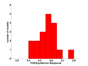 Histogram of the ratio of transient climate response (TCR) to equilibrium climate sensitivity in the 18 models for which both values are provided in Ch. 8 of the WG1/AR4/IPCC report
I find the following simple two degree-of-freedom linear model useful when thinking about transient climate responses:


The two box model reduces to the classic one-box model if 

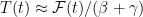
The equilibrium response in this model, the response eventually achieved for a fixed forcing, is 
These kinds of models are commonly used to help interpret the forced responses in much more elaborate GCMs. They are also often relied upon when discussing observational constraints on climate sensitivity. That is, one has a simple model with one or more parameters that control the magnitude of the response to a change in 
You can write down the solution to the two-box model, but let’s just look at the special case in which 

so the time scale of the response to an abrupt change in forcing is 

But now suppose that
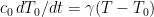
On these time scales both heat capacities drop out. The fast component is equilibrated, while the slow component is acting as an infinite reservoir. What is left is a response that is proportional to the forcing, with the deep ocean uptake acting as a negative feedback with strength 
The transient climate response, or TCR, is traditionally defined in terms of a particular calculation with a climate model: starting in equilibrium, increase 

The median of this ratio in the particular ensemble of GCMs referred to in the figure at the top of this post is 0.56. For several models the ratio is less than 0.5. Interestingly, it is very difficult to get ratios this small from the two-box model tuned to the equilibrium sensitivity of the GCMs and to their rate of heat uptake in transient simulations. (There is a fair amount of slop in these numbers — equilibrium responses are typically estimated with “slab-ocean” models in which changes in oceanic heat fluxes are neglected, and the transient simulations are single realizations — but I doubt that the basic picture would change much if refined.)
The heat uptake efficiency (


For the particular GCM CM2.1 discussed in post #3 (which has one of the smaller ratios of TCR to equilibrium response), using the numbers in that post,we need 


A few thoughts about heat uptake:
- Thinking linearly, when the system is perturbed, the unperturbed flow transports the perturbed temperatures, and the perturbed flow transports the unperturbed temperatures. Only if the former is dominant should we expect that the uptake to be proportional to the temperature perturbation. We might conceivably be able to think of the change in circulation as determined by the temperature response (if the changes in other things that affect the circulation, like salinities and wind stresses, can themselves be thought of as determined by the temperature field, but the circulation takes time to adjust and these time scales would destroy the simplicity of the intermediate regime if the circulation responses are dominant.
- Even if circulation changes are not dominant, the coupling to the deep oceans is strongest in the North Atlantic and the Southern Oceans, so the temperature anomalies in those regions presumably have more to do with the uptake than the global mean. Only if the forced warming is separable in space and time —
do we have any reason to expect the uptake to scale with the global mean temperature. A changing mix of greenhouse gas and aerosol forcing is the easiest way to break this separability.
- Do we have any simple theories explaining the rough magnitude of
[The views expressed on this blog are in no sense official positions of the Geophysical Fluid Dynamics Laboratory, the National Oceanic and Atmospheric Administration, or the Department of Commerce.]
Isaac – this is another interesting post for me! A quick question: roughly what deep-ocean timescale do you get by tuning the 2-box model to GCMs?
David
David — I wouldn’t take this two-box model that seriously. I use it here because it is the simplest model that interpolates between the short time limit in which the heat uptake is proportional to the temperature perturbation and the long time limit in which the heat uptake decays to zero. There are a lot of time scales involved in the oceanic adjustment. People often gravitate to simple diffusive models when emulating GCMs, even though diffusion is not a good description of what the ocean actually does, because it captures the idea that larger and larger reservoirs become involved at longer and longer times. In addition, on these slow oceanic adjustment time scales, the response to cooling is generally faster in models than the response to warming — because you are destabilizing the ocean in the former case, enhancing the vertical redistribution of heat — and this is not captured at all in the linear two-box model. See Stouffer (2004) for a description of the equilibration of the ocean in a GCM, illustrating some of these complexities. Having said all this, if you increase CO2 at 1%/year in CM2.1 until the time of doubling and then hold it steady, and ask how long it takes the global mean surface temperature to warm from its to
to  , I think it is about 400-500 years, keeping in mind that this global mean value is not very representative of particular regions.
Isaac – thanks. So your definition of the ‘intermediate regime’ is that range of timescales between a few years and these very long deep-ocean timescales? In particular the 70-year ramp-up time fits in here.
Does this post and your reply imply that, for practical purposes, is not a very useful measure of a climate model’s performance?
Sorry for these naive questions! I’m feeling my way into the topic…
David, no need to apologize; you are going straight towards the question that I am dancing around. But to define “practical purpose” would take us outside of climate science, and therefore outside of the space I would like to keep this blog confined to. The key question is whether nature has as sharply defined an intermediate regime as do some of our climate models.
I’ve often used the 2-box model to fit forcing to observed global temperature data. I find that the fast response may be even faster than the 4-yr time scale suggested. In fact I’ve found a good match using a very short (less than 1 year) response and a second time constant of about 14 years (but I’ll soon be fitting some new forcing data I’ve acquired, and will probably get different results). I recognize that fitting estimated forcing to global temperature anomaly limits me to a little over a century of data, which precludes exploring very long time scales (i.e., the 400-500 years indicated by your model). Perhaps we should try a 3-box model?
Doesn’t the lag between land surface temperature and the seasonal cycle, as well as the hemispheric difference in temperature trend, argue for less than a 4-year time scale for one of the boxes? I know that the atmosphere/land surface has a much lower specific heat than even a modest ocean slab, but doesn’t it also has a disproportionate impact on surface air temperature (esp. over land)?
Tamino,
I have enjoyed reading your analyses of climatic time series.
1) the long time scale:
Putting aside glaciers and the carbon cycle and just focusing on physical coupled atmosphere-ocean models, the TCR is always substantially smaller than the equilibrium sensitivity, as indicated in the figure for the CMIP3 models. You can’t get this without time scales much longer than 14 years. Ignoring this point results in a lot of confusion as to what the models are predicting — ie “how can equilibrium sensitivities of 3K possibly be consistent with the observed warming to date?” It’s not an easy time scale to get at with the instrumental record.
2) the short time scale:
I was working with annual mean forcing and model temperatures, effectively filtering out shorter time scales. There is a very fast atmospheric/land response to impulsive forcing and to the seasonal cycle. But a time scale around 4 or 5 years seems to me to be unavoidable, as this is roughly the relaxation time of the oceanic mixed layer. I think it’s hard to get this time scale up to 14 years. Time scales of 10-50 years could come from relatively shallow oceanic circulations, but this is also where uncertainty in the forcing and the potential for internal variability on multi-decadal time scales comes into play when fitting observations.
Emulating GCMs with simple models and then comparing these simple models with observations is a rather indirect way of comparing GCMs to observations — but I think it can be very useful in communicating and getting a feeling for what the models are saying. So it is interesting to see how much one has to tweak forcing, and/or the magnitude of unforced variability, to make a case for consistency of this GCM-motivated simple model (a 4 year time scale and a multi-century time scale) with observations.
Dr Held,
I think you may have some fun with me, I have posted on the simplicity thread and reading the above I can see that I will play simplicity as a high valued card.
I respect your detailed knowledge of the subject but I am going to suggest that it goes against acting in the most simple manner.
You understand the requirements of even a simple model to be a representation of known physical properties. I feel I am going to argue that this detracts from the formulation of modelling to emulate observations under the guidance of the keep it simple imperative.
I have some notion of the properties of the surface mixed layer but I do not feel hampered by this to produce of an emulator that has such knowledge built in. If the output I wish to model is as well or better emulated with an unphysically thin SML over an upwelling diffusive ocean I should model it that way. If I find that the monthly variance is compatible with a diffusive model because a SML of physical proportions attenuates monthly temperature variance too much I would prefer an unphysically thick layer. Also if I find that the SST spectra of the real world and importantly the models is more closely pink (diffusive) rather than red (slab) like I would choose a diffusive emulation even though it might be an inexplicable choice viewed from a position of greater real world knowledge.
I think some of the issues you comment on here are actually well covered by the diffusive emulation assumption, namely different time constants for short and long term considerations, plus others like monthly variance and the famous long tail to equilibrium, these are emulated by the upwelling diffusive model naturally without having to resort to a handfull of different time constants. This is not saying that such time constants are invalid, only that if they are adequately and indistinguishably covered by a diffusive emulator that has just a single ocean parameter then the why not just use the simpler form and just whence that it defies wisdom.
Now I think I could show that a diffusive emulation touches all the bases rather well.
It predicts the following:
That phase angles will tend to a fixed value around pi/2 for cyclic phenomenon, that is phase lags will scale with period. The seasons shifted by around 50 days, the solar ripple by around 1.5 years, neither are quite the accepted values perhaps but they a natural scaling is evident without recourse to separate time constants.
That the OHC will have a certain form derivable from the surface temperature that is quite distinct from, and I would argue more realistic than, that produced by a SML slab. Now wisdom might prevail to say that this is the wrong way to try and derive OHC, but simplicity argues that an emulator’s job is to emulate not to be unnecessarily realistic in physical terms.
That long term variability will be higher than that for slab models, and hence some phenomenon such as small but significant looking wobbles like the PDO may be just happenstance and for them to be absent would be a surprise. Again I ignore that the PDO probably has some understood structure but if the amount of variance produced is within the scope of an emulation that lacks such subtleties were is the harm.
I could, and eventually will go on.
Anyway I hope I have amused rather than insulted. My position is that over burdening an emulation with knowledge that goes beyond its remit can be counter-productive.
Alex
I am pleased that you have chosen to blog on climate science. I have often argued that the participation of working climate scientists is very important to help resolve politically motivated conflicts related to global warming and consequences of global warming.
With regard to equilibrium versus short term responses to forcing, there seems to me to be quite a lot of uncertainty in ocean heat accumulation rates. Lyman et al’s estimate of ~0.64 watt per M^2 appears due mainly to a rapid run-up in near-surface ocean heat accumulation (associated with a rising overall global trend) between 1993 and about ~2002; recent warming (especially since the Argo deployment was completed) suggests a substantially lower rate of warming. When you consider the relative quality of the pre-Argo versus post Argo data (and the odd looking apparent step-change at the transition, https://www.nodc.noaa.gov/OC5/3M_HEAT_CONTENT/ it seems clear that ocean heat accumulation rate is much less than very certain. The best estimate of post 2004 ocean heat accumulation is very low compare to 1993 -2003.
If in fact there is a large surface temperature lag to forcing associated with ocean heat accumulation, I would never expect there to be a rapid transition from substantial accumulation to very little accumulation. The observed change in rate of accumulation over a relatively short time indicates (to me at least) that the 0-700 meter heat content tracks surface temperate quite closely, and that the difference between current and equilibrium warming is modest.
Steve, I have a tendency to oversimplify, so thanks for the corrective. There are a lot of issues with regard to the ARGO vs XBT data sets, consistency with sea level trends, uncertainty about the contribution from layers below those typically considered in these estimates (700m in Lyman et al), whether models can generate relatively flat heat content for 5 or 6 years in the upper 700 m, through internal variability and in the absence of volcanoes (as has evidently been the case in the most recent period), etc. If the (surface) climate is in fact closer to equilibrium than typical GCMs suggest, this would require a reduction in estimates of sensitivity, with fixed forcing, to maintain consistency with 20th century warming. Nothing can be more fundamental to our understanding of climate change.
But it is also important to realize that mixing/transport from shallow to deeper layers in ocean models is tested against observations in other ways — comparison with data collected in recent decades on the slow penetration of CFCs into the oceans is one of the best examples — try googling “CFCs in the ocean” if unfamiliar with this topic. Which is not to say that CFC simulations don’t have issues, but that data relevant to evaluating ocean mixing in models can come from sources other than just the heat content data itself.
Issac,
Thank you for your thoughtful reply.
I completely agree that there are other measures of mixing in the ocean surface layers, including, of course, CFC and C14 penetration into the ocean surface and deep convective layers; like all measures of ocean mixing, CFC (and radio carbon) have considerable associated uncertainties. My comment was mainly made to point out that the bulk of the data on hand, and associate uncertainties, does not very well constrain net climate sensitivity. My hea balance analysis (perhaps naive) of this issue is simple: I look at the credible level of ocean heat accumulation at all depths (currently perhaps ~0.35 watt per square meter, with some uncertainty, of course), the best estimates of radiative forcing (~3.0 watts per square meter), and then consider what a range of credible aerosol offsets imply for long term climate sensitivity.
As best I can figure, the credible range of man-made aerosol off-sets (IPCC) is ~0.5 watt per square meter to ~2 watts per square meter. Assuming:
1) a global temperature rise of 0.85C from pre-industrial times until now,
2) current GHG radiative forcing of ~3 watts per square meter, and
3) 100 % of warning since the pre-industrial period is due to GHG forcing
then if the above are correct (and there is no certainty of that!) I estimate the true equilibrium sensitivity must lie between ~1.47 C per doubling and ~4.85 C per doubling (of CO2).
Of course, if any of the rise in temperature from the preindustrial period to present was in fact due to causes other than GHG forcing, then the net sensitivities would have to be reduced to somewhere below the above estimated , indeed, overwhelming range of net sensitivities.
So, here (for me) is the issue: the credible range of sensitivities, considering the basic heat balance, covers anything from “not very important’, to ‘alarming’.
Determining (with reasonably high confidence) the actual sensitivity to GHG forcings is the most important question facing climate science, and one that dominates all other issues.
I was greatly saddened by the recent loss of the Glory satellite, since this failure appears to blind us on crucial aerosol effects for many years to come.
Steve, Isaac,
Just a thought on the extent to which we can look at recent changes in heat content to determine whether they have kept pace or not with surface temperature changes. Even though since 2003 we are in an exciting time with what is unarguably the densest sampling of the ocean (through ARGO, satellites and the other elements of the global climate observing system), the observations and our tools to analyze those observations are perhaps still not at the stage where we can be confident in the sign – much less the magnitude – of recent heat content changes.
Table 1 of Chang et al (2010, J. Marine Systems) provides an estimate of 2003-2007 trends in global steric height change (a measure of the average density of the ocean, which is strongly connected to heat content changes, increasing steric sea level indicates warming) and compares to three other recent estimates, each using similar raw data, but analyzing (filling holes, etc) them slightly differently (Willis et al 2008, J. Geophys. Res.; Leuliette and Miller 2009, Geophys. Res. Lett.; Cazenave et al. 2009, Glob. Planet. Change). One of the studies finds a negative trend (-0.5 +/- 0.5 mm/year), one finds no significant change (-0.11 +/-0.22 mm/year), and two find positive trends (+0.8+/-0.8 mm/year and +0.37+/-0.1 mm/year). Notice that the error bars of the different studies barely overlap. I think the Lyman et al (2010) results would fall somewhere near “no change”.
Therefore, I’d be cautious about over-interpreting the results from any single study, since even with a dense sampling network differences in the way the data are analyzed can lead to different signs – never mind magnitudes – of ocean heat content changes. Also, it’s worth noting that these studies I mentioned focus primarily on heat content changes in the upper 700-1000 meters of the ocean, and changes in the deep ocean are less well known; the recent Purkey and Johnson (2010, J. Climate) paper suggests that global ocean warming below 4000 meters and Southern Ocean warming between 1000-4000m could account for an additional 0.1 W/m2 over the 1990-2000s.
As Isaac’s post and your comments indicate, this uncertainty in what recent heat content changes have been touches upon a very important open question in climate science. Hopefully with continued years of sampling and improvements in our understanding of how best to analyze the data we will soon be in a position to better bound the possibilities.
Gabriel,
Thanks for the link to Chang et al. I will read this over the next couple of days. I have already read the other papers.
I completely agree that individual estimates of heat accumulation should be viewed with considerable caution, especially considering that the individual uncertainty ranges sometimes do not even overlap; something is clearly amiss. There must be other substantive issues to be resolved, and it appears that any short term trend may not be at all representative of a longer term trend.
But in spite of this, one common constraint is the measured sea level. The trend is remarkably constant since 1993 for any period longer than a few years. Substantial unaccounted changes in heat accumulation seem to me unlikely, unless you want to argue that other water volume sources (mountain glacial melt, Greenland, etc.) have happened by chance to compensate for variations in steric volume growth.
Issac apologies but I have a rather simplistic question.
Is the rapid rise in OHC from 2002-2004 physically realistic? To put it another way how would you account for it as a real world phenomenon? It seems to account for close to half of the heat accumulation in the Lyman period.
http://static.skepticalscience.com/images/robust_ohc_lyman2.gif
I’ve read from various sources
1) That OHC suffers less than other metrics from interannual variability. I’ve read this as a defence of Hansen’s decadal prediction of climate sensitivity. It also seems to be supported by the short ARGO data set.
https://pielkeclimatesci.files.wordpress.com/2011/03/roger_ohc.gif
2) That a data artifact maybe a better explanation for the observed rise.
3) There appears to be no obvious reason for the rapid rise (no volcano, no strong ENSO event etc.)
I think it is fair to say that the big picture that I am trying to paint is more dependent on the longer term trends than on these higher frequencies (whether real or artifacts). The problem of getting tight and consistent observational constraints on energy budgets over the relatively short time scales that you are focusing on is not going to be solved quickly.
Something to keep in mind: if your reduce and increase
  , holding their sum fixed, you do not change the response as long as you are in what is referred to in the post as the “intermediate regime” — in particular, although you would be reducing the equilibrium climate sensitivity, you wouldn’t be changing the TCR very much. So to the extent that you can think of
  as constrained by the observed warming over the past century (and estimates of the forcing), you are not going to be changing your projection of the forced response much over, say, the next half century.
Isaac, thank you very much for taking the time to post these articles, they are very insightful & interesting.
Regarding your Figure 1, I was curious whether you have the following figures, or know of a reference that shows them,
1) scatter plot of TCR/TEQ versus ECS.
2) modeling “settling time” to reach TEQ versus ECS.
I’d guess that TCR isn’t very different between models and that the main difference is in ECS, and I’d also guess that models with high values of ECS have longer response times to reach equilibrium.
Thanks for any help!
Carrick
Not sure what distinction you are making between ECS and TEQ — ignoring this distinction — I am not familiar with a plot of TCR/TEQ vs TEQ, but you can make one yourself from the table in Winton et al 2010 for CMIP3 most of which is taken from a table in AR4. While one might guess that TCR has less variation across the CMIP ensembles that TEQ, at least from the numbers in this table one finds that the coefficient of variation for TCR is similar to that for TEQ. These numbers are not as precise as one would like them to be — estimates of TCR are often based on single realizations, and TEQ based on extrapolation.
Taking the 2-box model (with negligible deep ocean warming) at face value one gets .
.
Thanks, that’s very interesting.
If I fit to TCR/TEQ = 1/(a + b TEQ), I get a = 1.03±0.28 and b = 0.26±0.08, p = 0.0042