

Posted on April 10th, 2013 in Isaac Held's Blog
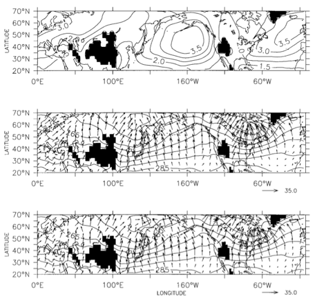 Lower panel: the observed (irrotational) component of the horizontal eddy sensible heat flux at 850mb in Northern Hemisphere in January along with the mean temperature field at this level. Middle panel: a diffusive approximation to that flux. Upper panel: the spatially varying kinematic diffusivity (in units of
Let’s consider the simplest atmospheric model with diffusive horizontal transport on a sphere:

Here 


We can choose

(Corrected sign errors — Aug 2013). If we are using this equation to model the time averaged north-south temperature gradients we can think of
We can talk about an atmospheric radiative relaxation time scale, 


The bottom panel in the figure at the top is the eddy sensible heat flux, 

(Actually, before plotting the flux, we decompose it into a a part that has zero divergence on this surface and a part that has zero curl –this Helmholtz decomposition is unique on the sphere– and retain only the latter part, since we are only interested in the divergence of the flux here. If you don’t do this, the flux is not as cleanly directed downgradient.)
The fluxes in the middle panel are generated with the same mean gradients and with the spatially varying diffusivity shown in the upper panel. The result is evidently in the right ballpark. The kinematic diffusivity has the dimensions of (length)2/(time), or velocity times length. One could try to develop a theory for the relevant length and time scales or one could estimate them from observations in different ways. Here we do the latter, and take the shortcut of just looking at the streamfunction of the flow. The atmospheric flow is approximately non-divergent in the horizontal, so can be described by a streamfunction 


A fascinating question for me, ever since I entered the field, is how the magnitude and structure of this diffusivity is determined. (In Held 1999, I discuss why turbulent diffusion might actually be a better approximation for the atmosphere, at least for the transport of sensible heat in the lower troposphere, than for typical shear or convectively driven turbulence studied in the laboratory.) We expect this effective diffusivity to change as the climate changes, since the diffusivity must be determined by some aspect of the large-scale environment giving rise to these storms. In particular, most theories have this diffusivity increasing with the magnitude of the north-south temperature gradient, making it harder to change this gradient than one might otherwise guess.
The values of the diffusivity in the middle of the oceanic storm tracks rise above 

But my motivation in bringing up this topic is a concern about the opposite tendency to ignore the difficulty that the atmosphere has in communicating temperature responses from extratropical latitudes of one hemisphere to extratropical latitudes of the other. A diffusivity of 2-3 x 10⁶ m2/s, if uniform over the sphere, is not large enough to mix from pole to pole in an atmospheric radiative relaxation time. The effective diffusivity gets small as one enters the tropics — one can see a bit of this reduction in the figure — seemingly making it harder still to communicate between hemispheres, but this is potentially misleading because the large scale overturning (the “Hadley Cell”) is very efficient at destroying temperature contrasts across the tropics. This effect is sometimes mimicked in diffusive models by using a large diffusivity in the tropics, which can be confusing since this diffusivity would not be relevant for passive tracers. In addition the strong tendency for the tropical circulation to wipe out horizontal temperature gradients applies to deep temperature perturbations in the free troposphere, from which the surface can be protected by structure in the atmospheric boundary layer. In any case, the signal still has to move through the tropics, which provide a large area to radiate it away to space, so the difficulty in getting much of a signal to reach extratropical latitudes in the opposite hemisphere remains. GCMs provide an essential tool for navigating this complexity. (But uncertain cloud feedbacks, the familiar wild card when discussing global sensitivity, can also come into play in this problem.)
When thinking about aerosol forcing, which is heavily tilted to the Northern Hemisphere, no one is surprised if the response is strongly tilted to the Northern Hemisphere as well. But consider the concept of (global mean) transient climate response (TCR), discussed in several earlier posts. The TCR is dependent on the efficiency of heat uptake by the oceans. Much of this heat uptake occurs in the North Atlantic and in the Southern Ocean. Consider two models, identical except for the Southern Ocean heat uptake. The one that warms more slowly in the Southern Ocean will have a smaller TCR, which is fine, but would the warming in the extratropical Northern hemisphere be substantially smaller? I don’t think so. I am not aware of a simulation addressing this specific question in the literature.
A paper by Stouffer 2004 (Fig 5 in particular) is informative. This paper describes very long simulations of the response to doubling and halving of CO2 in a coupled atmosphere-ocean model (5,000 years — long enough for this model to approach its new equilibrium quite closely ). In the 2 x CO2 case at year 200 the Southern Hemisphere (SH) as a whole, held back in large part by the Southern Ocean, has reached about 40% of its final temperature response. Meanwhile the Northern Hemisphere (NH) has achieved over 80% of its equilibrium response. Even if all of the NH disequilibrium is due to the lack of warming in the Southern Hemisphere, which is unlikely, there is little room left for the rest of the SH warming to affect the NH — implying that a change in the SH relaxation time would have only a small effect on the NH in this model.
Thinking in terms of the global mean temperature in isolation can be valuable and it can also be misleading. I tried to argue in Post #7 that neither of the usual arguments for focusing on the global mean — reduction in noise and the connection to the global mean energy balance — is very compelling. (To think about one way in which the energy balance can get divorced from the mean temperature, just make 
(Thanks to Sarah Kang, Paulo Ceppi, Yen-Ting Hwang and Dargan Frierson for discussions on closely related topics.)
[The views expressed on this blog are in no sense official positions of the Geophysical Fluid Dynamics Laboratory, the National Oceanic and Atmospheric Administration, or the Department of Commerce.]
Isaac,
Thanks for this post.
I think it would also be interesting to change the spatial structure of the heat uptake (e.g., put a “Southern Ocean” in the tropics) to look at TCR and its spatial and time distribution. Are you aware of idealized modeling that has looked at this?
There is quite a bit of work using aqua-planet models coupled to slab oceans, perturbing them with heat input/output from the slab with different patterns. These are not focused specifically on TCR but from a linear perspective this is pretty much the same thing. My own work along these lines, in collaboration with Sarah Kang primarily, has mostly been focused on circulation responses, how extratropical perturbations alter the tropical circulation, rather than surface temperature, ie Kang et al 2008. Looking at transient responses in a fully coupled comprehensive model and then somehow manipulating it to change the distribution of the heat uptake in some region is more difficult.
As I noted in a comment on one of the previous posts I was impressed by an as yet unpublished (?) paper by your collaborator Kang (with Seager), “Croll Revisited” relating to inter-hemispheric oceanic heat transport. It would be interesting to compare that with the model used in Stouffer 2004.