

Posted on June 14th, 2013 in Isaac Held's Blog
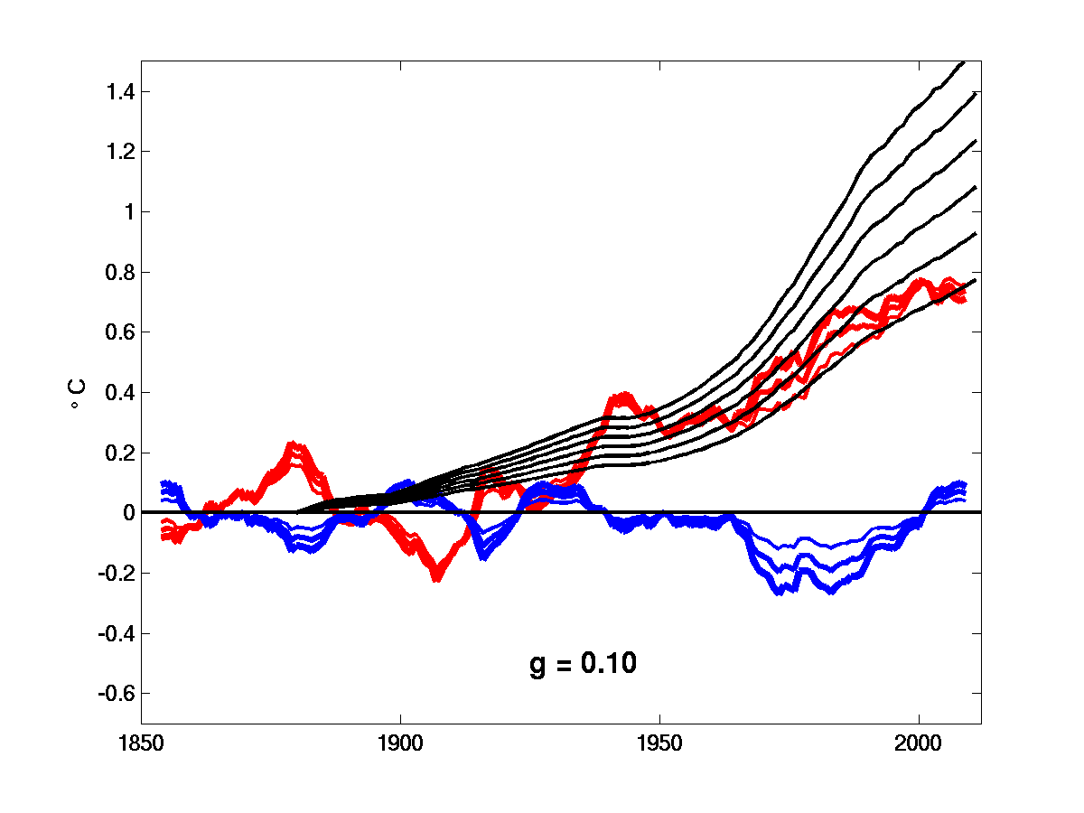
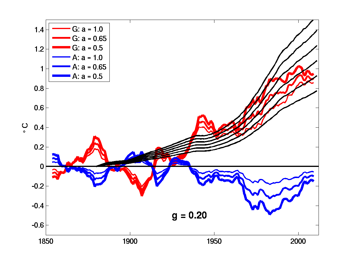
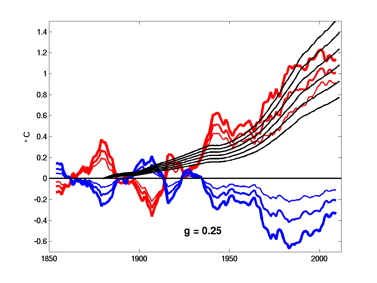 Rough estimates of the WMGG (well-mixed greenhouse gas — red) and non-WMGG (blue) components of the global mean temperature time series obtained from observed (HADCRUT4) Northern and Southern Hemisphere mean temperatures and different assumptions about the ratio of the Northern to Southern Hemisphere responses in these two components. Black lines are estimates of the response to WMGG forcing for 6 different values of the transient climate response TCR (1.0, 1.2, 1.4, 1.6, 1.8, 2.0C).
How can we use the spatial pattern of the surface temperature evolution to help determine how much of the warming over the past century was forced by increases in the well-mixed greenhouse gases (WMGGs: CO2, CH4, N2O, CFCs), assuming as little as possible about the non-WMGG forcing and internal variability. Here is a very simple approach using only two functions of time, the mean Northern and Southern Hemisphere temperatures. (See #7, #27, #35 for related posts.)
Suppose that the temperature record consists of the linear superposition of two parts — the WMGG part and everything else. The real distinction here is that these two parts are assumed to affect the Northern and Southern Hemispheres differently. If the global mean response to the WMGG is G(t), assume that the Northern and Southern hemisphere responses are respectively (1+g)G and (1-g)G. Similarly for the non-WMGG part, A(t), I’ll write the two hemispheric responses as (1+a)A and (1-a)A. Here the constants g and a, controlling the pattern of the responses, are assumed to be independent of time, so that the two parts of the response are individually separable in space and time. Given the Northern and Southern hemisphere mean temperatures, N(t) and S(t), I’ll just write
N(t) = (1+g)G(t) +(1+a)A(t),
S(t) = (1-g)G(t)+(1-a)A(t).
Assuming g and a are given we can solve for the global mean responses G and A:
G(t) =- [(1-a)*N(t) – (1+a)*S(t)]/(2*(a-g)),
A(t) = [(1-g)*N(t) – (1+g)*S(t)]/(2*(a-g)).
For example, in the special case of a=1 — in which the non-WMGG part is confined to the Northern Hemisphere — then G = S/(1-g) — so the WMGG component is determined completely by the Southern Hemisphere only, being uncontaminated by the non-WMGG component there.
 Using N(t) and S(t) from HadCRUT4.2.0.0 and varying g and a over ranges of interest I get the figures at the top. Anomalies are computed from the mean of the first 60 years, starting in 1850, and smoothing with a running 9 year average. (See figure immediately above.) Each panel in the figure at the top of the post corresponds to one value of g (top: g = 0.10; mid: g = 0.20; bot: g = 0.25) and G(t) and A(t) are shown for three different values of a (0.5, 0.65, and 1.0 as indicated by the legend on the middle panel — the three values of a are the same in each panel ). Also shown is the response to WMGG forcing using the GISS forcing estimate, normalizing by a multiplicative constant to agree with the value of Skeie et al 2011 of 2.83 W/m2 in 2010, and then multiplied by (TCR)/(2xCO2), where (2xCO2) = 3.7 W/m2. The 6 black lines in the figure correspond to TCR = {1.0, 1.2, 1.4, 1.6, 1.8, 2.0}. If you can ignore phase lags between forcing and response, you can think of TCR (the transient climate response) in this context as the just a multiplicative constant that you multiply the WMGG forcing by to get the global transient climate response to the WMGGs, in degrees C, normalized to refer to doubling of CO2. The TCR implicitly takes into account ocean heat uptake as well as radiative feedbacks and (I feel that I have to repeat this whenever using this concept) should not be confused with the more familiar “climate sensitivity”, which requires the oceans to have equilibrated and the ocean heat uptake to relax to zero.
One can read off the value of g simulated by a set of CMIP5 models run with varying WMGGs as the only forcing agents in Fig. 4 of Friedman et al 2013. I get about 0.15 or 0.20 eyeballing the figure. Also, if you assume that the non-WMGG component is primarily aerosol forced, the same figure implies a value of a of about 0.5 . (The figure also gives you a sense of how separable in time the responses are to WMGGs and aerosols in isolation.) If mutidecadal natural variability dominates over aerosols, then I would expect a value of a closer to 1, or even greater than 1, since variability in the Atlantic overturning, in particular, should, if anything, cool the southern while warming the northern hemisphere. ( If the non-WMGG component consists of an aerosol part and an interannual variability part of comparable magnitude, and with different values of a, this kind of simple linear transformation will be of limited utility.) If there are other forcing agents (ie increased stratospheric water or tropical volcanoes) that result in a modest interhemispheric contrast in warming or cooling similar to the assumed structure of the WMGG response, these would find themselves lumped together with the WMGG component. You don’t have to smooth, but interannual variability (ie ENSO) most likely would not project cleanly onto one or the other component, so I don’t see any advantage of leaving it in.
I have used these numbers and considerations in deciding which combinations of (g,a) to use in the plots, also keeping in mind that it makes no sense to allow g and a to get too close to each other, since the near-degeneracy would then result in a meaningless decomposition.
The idea here, which should be clear from the inclusion of the TCR-normalized WMGG forcing curves in the figures, is to use what we are relatively sure about — the time history and the radiative forcing from the WMGG’s — to constrain TCR. while assuming as little as possible about aerosol forcing and natural multi-decadal variability.
The panel at the top is a case with g approaching 0. In this limit the non-WMGG component has to explain all of the interhemispheric difference, and since this component is assumed to be Northern-centric the observed larger increase in the north requires global mean warming from this term, pushing the WMGG component down to a TCR value of 1.0 or so. This is a picture that you might favor if you think, for other reasons, that the non-WMGG component is dominated by internal variability.
The middle panel has somewhat larger TCR, with the net non-WMGG component small near the present because the observed north/south ratio is similar to that implied by the assumed WMGG pattern in isolation.
In the bottom panel, the value of g is large enough to leave room for a substantial “aerosol” affect remaining at present, resulting in a larger TCR that depends more strongly on the value of a: a smaller a results in less difference in the north-south ratios between the two patterns, producing more compensation.
These results will be sensitive to the input data set due to the role played by the relatively small interhemispheric differences. You could propagate the observational error estimates provided along with the HADCRUT4 data set through this transformation, as well as use information about the distribution of a and g from individual models in the CMIP ensembles. But the choice of the two hemispheric means for this analysis is arbitrary. I am sure that one could be more systematic along the lines of the fingerprinting literature (but much of this literature assumes more about the aerosol forcing time dependence than I would prefer). And one could look in more detail at the assumption of negligible phase lag in the WMGG response over the past century needed when trying to constrain TCR. I am thinking of this as being more exploratory than quantitative, nudging readers of this blog to think beyond the global mean time series.
[The views expressed on this blog are in no sense official positions of the Geophysical Fluid Dynamics Laboratory, the National Oceanic and Atmospheric Administration, or the Department of Commerce.]
So if I understand your comments correctly, you are estimating a TCS of about 1.3C. Is that right?
That is the neighborhood suggested by this manipulation. But there are a lot of assumptions built in. To the extent that there are models that fit both NH and SH temperatures well and have TCRs greater than 1.8 or so, we should be able to learn something by thinking about why this argument does not apply to those models.