

Posted on June 7th, 2015 in Isaac Held's Blog
Given the problems that our global climate models have in simulating the global mean energy balance of the Earth, some readers may have a hard time understanding why many of us in climate science devote so much attention to these models. A big part of the explanation is the quality of the large-scale atmospheric circulation that they provide. To my mind this is without doubt one of the great triumphs of computer simulation in all of science.
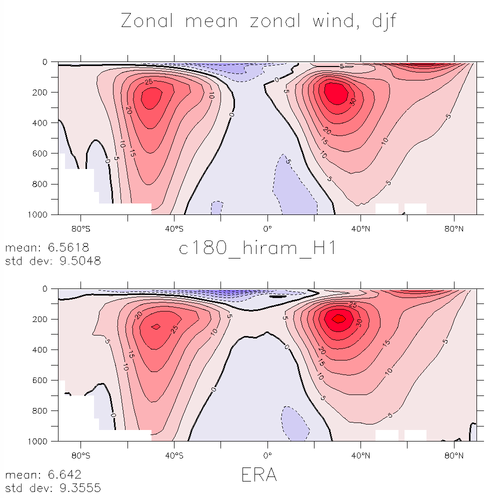
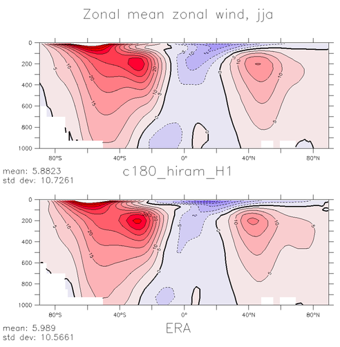
The figure above is meant to give you a feeling for this quality. It shows the zonal (eastward) component of the wind as a function of latitude and pressure, averaged in time and around latitude circles. This is an atmosphere/land model running over observed ocean temperatures with roughly 50km horizontal resolution. The model results at the top (dec-jan-feb on the left and june-july-aug on the right) are compared with the observational estimate below them. The observations are provided by a reanalysis product(more on reanalysis below). The contour interval is 5m/s; westerlies (eastward flow) are red, easterlies are blue. Features of interest are the location of the transition from westerlies to easterlies at the surface in the subtropics, and the relative positions of the the subtropical jet at 200mb, the lower tropospheric westerlies and the polar stratospheric jet in winter (the latter is barely visible near the upper boundary of the plot when using pressure as a vertical coordinate).
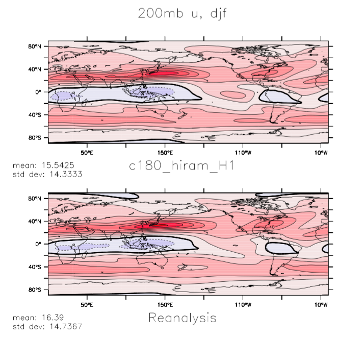
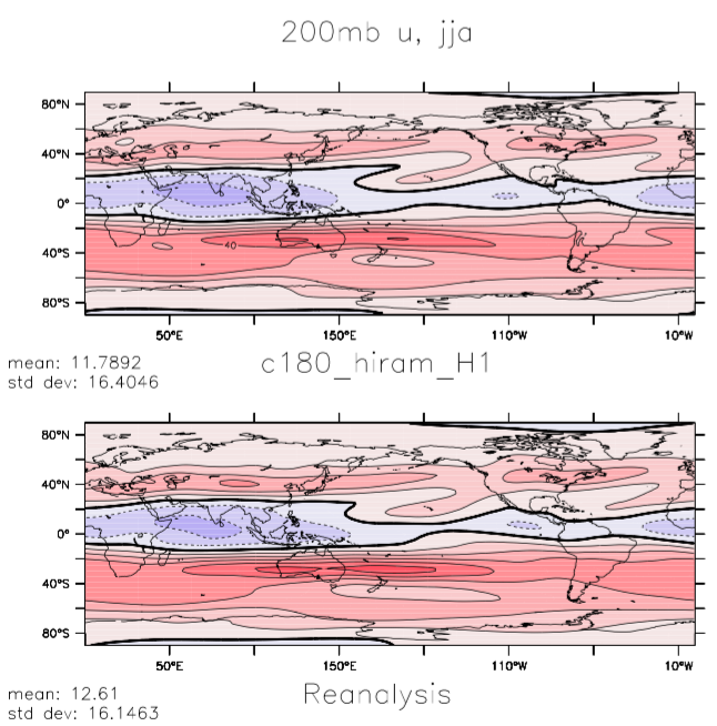
The next plot is also of the zonal component of the wind averaged over the same two seasons, but now on the 200mb surface, close to the subtropical jet maximum near the tropopause. Features of interest here include the orientations of the Pacific and Atlantic jets in the northern winter (models often have difficulty capturing the degree of NE-SW tilt of the Atlantic jet) the secondary westerly maxima over the northern tropical oceans in northern summer (time-mean signatures of the tropical upper tropospheric troughs — TUTs) and the split in the jet over New Zealand in southern winter. The contour interval here is 10m/s.
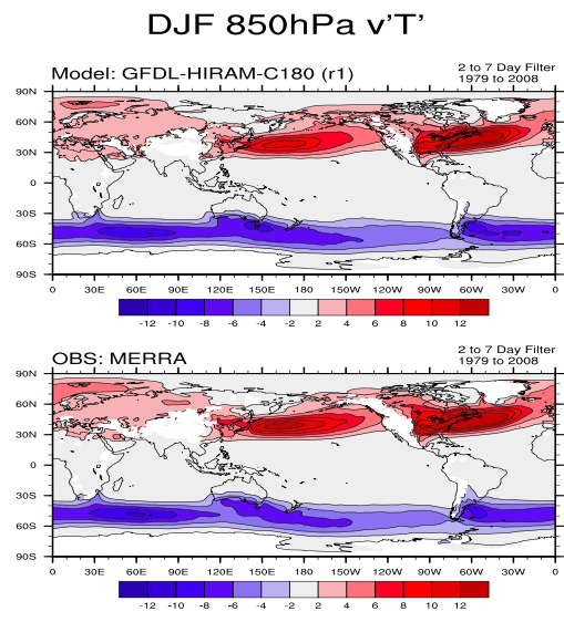
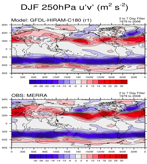
This circulation cannot be maintained without realistic simulation of the heat and momentum fluxes due to the dominant eastward propagating midlatitude storms familiar from weather maps. These fluxes depend not just on the magnitude of these eddies but also the covariability of the eastward component of the wind (u), the northward component of the wind (v), and the temperature (T). The following plot, focusing on the winter only, shows maps of the northward eddy heat flux, the covariance between v and T, and the eddy northward flux of eastward momentum, the covariance between u and v. The latter, in particular, turns out to be fundamental to the maintenance of the surface winds and can be challenging to capture quantitatively. The plots show these fluxes only for eddies with periods between roughly 2 and 7 days (fluxes due to lower frequencies are also significant but have different dynamics and structures.) Each flux is shown at a pressure level close to where it is the largest: the eddy heat flux is largest in the lower troposphere, while the momentum fluxes peak near the tropopause. The storm tracks, marked by the maxima in the down-gradient poleward eddy heat fluxes in the lower troposphere, are accompanied by a dipolar structure of the momentum fluxes in the upper troposphere, with meridional convergence of eastward momentum into the latitude of the storm track. The eddies responsible for these fluxes have scales of 1,000 km and greater. This is what we mean by the term large-scale flow in this context.
I am using reanalysis as the observational standard for these fields, an idea that takes some getting used to. Weather prediction centers need initial conditions with which to start their forecasts. They get these by combining information from past forecasts with new data from balloons, satellites, and aircraft. These are referred to as analyses. If you took a record of all of these analyses as your best guess for the state of the atmosphere over time, it would suffer from two inhomogeneities — one due to changes in data sources and another due to changes in the underlying model that the data is being assimilated into. Reanalyses remove the second of these inhomogeneities by assimilating an entire historical data stream into a fixed (modern) version of the model. They still retain the inhomogeneity due to changing data sources over time. Where data is plentiful the model provides a dynamically consistent multivariate space-time interpolation procedure. Where data is sparse, one is obviously relying on the model more.
The multivariate nature of the interpolation is critical. As an important example, horizontal gradients in temperature are very closely tied to vertical gradients in the horizontal wind field (for large-scale flow outside of the deep tropics). it makes little sense to look for an optimal estimate of the wind field at some time and place without taking advantage of temperature data. The underlying model and the data assimilation procedure handle this and less obvious constraints naturally. Importantly, the model can propagate information from data rich regions into data poor regions if this propagation of information is fast enough compared to the time scale at which errors grow. For climatological circulation fields such as the ones that I have shown here reanalyses provide our best estimates of the state of the atmosphere. For the northern hemisphere outside of the tropics these estimates are very good — I suspect that they provide the most accurate description of any turbulent flow in all of science. For the tropics and for the southern hemisphere the differences between reanalyses can be large enough that estimating model biases requires more care.
I am claiming that the comparison to reanalyses is a good measure of the quality of our simulations for these kinds of fields. (You need to distinguish estimates of the mean climate described here from estimates of trends, which are much harder.) If you accept this then I think you will agree that the quality seen in the free-running model (with prescribed SSTs) is impressive (which does not mean that some biases are not significant, for regional climates especially). This quality is worth keeping in mind when reading a claim that atmospheric models as currently formulated are missing some fundamentally important mechanism or that the numerical algorithms being used are woefully inadequate.
I would also claim that these turbulent midlatitude eddies are in fact easier to simulate than the turbulence in a pipe or wind tunnel in a laboratory. This claim is based on the fact the atmospheric flow on these scales is quasi-two-dimensional. The flow is not actually 2D — the horizontal flow in the upper troposphere is very different from the flow in the lower troposphere for example — but unlike familiar 3D turbulence that cascades energy very rapidly from large to small scales, the atmosphere shares the feature of turbulence in 2D flows in which the energy at large horizontal scales stays on large scales, the natural movement in fact being to even larger scales. In the atmosphere, energy is removed from these large scales where the flow rubs against the surface, transferring energy to the 3D turbulence in the planetary boundary layer and then to scales at which viscous dissipation acts. Because there is a large separation in scale between the large-scale eddies and the little eddies in the boundary layer, this loss of energy can be modeled reasonably well with guidance from detailed observations of boundary layer turbulence. While both numerical weather prediction and climate simulations are difficult, if not for this key distinction in the way that energy moves between scales in 2D and 3D they would be far more difficult if not totally impractical.
I have been focusing on some things that our atmospheric models are good at. It is often a challenge to decide the relative importance, for any aspect of climate change, of the parts of the model that are fully convincing and those that are works in progress, such as the global cloud field or specific regional details (you might or might not care that a global model produces a climate in central England more appropriate for Scotland). You can err on the side of inappropriately dismissing model results; this is often the result of being unaware of what these models are and of what they do simulate with considerable skill and of our understanding of where the weak points are. But you can also err on the side of uncritical acceptance of model results; this can result from being seduced by the beauty of the simulations and possibly by a prior research path that was built on utilizing model strengths and avoiding their weaknesses (speaking of myself here). The animation in post#2 is produced by precisely the model that I have used for all of the figures in this post. I find this animation inspiring. That we can generate such beautiful and accurate simulations from a few basic equations is still startling to me. I have to keep reminding myself that there are important limitations to what these models can do.
[Note added June 10 in response to some e-mails. For those who have looked at the CMIP archives and seen bigger biases than described here, keep in mind that I am describing an AMIP simulation — with prescribed SSTs. The extratropical circulation will deteriorate depending on the pattern and amplitude of the SST biases that develop in a coupled model. Also this model has roughly 50km horizontal resolution, substantially finer than most of the atmospheric models in the CMIP archives. These biases often improve gradually with increasing resolution. And there are other fields that are more sensitive to the sub-grid scale closures for moist convection, especially in the tropics. I’ll try to discuss some of these eventually.]
[The views expressed on this blog are in no sense official positions of the Geophysical Fluid Dynamics Laboratory, the National Oceanic and Atmospheric Administration, or the Department of Commerce.]
If I understand correctly, re-analyses are constructed by constraining the output from a climate or weather models to agree with observational data. In the case of wind speed, that data may come from radiosondes, i.e. mostly over land in the Northern Hemisphere. Do you have any idea to what extent the details in the “observations” represent the “proclivities” of the model used in the re-analysis and to what extent those details are defined by observational data. If you calculated the difference between the model output and the re-analysis and found/didn’t find the greatest disagreement in areas with the best observational data, you might have a better idea of the importance of the agreement discussed in this post. Comparing one re-analysis to another might also be informative.
Comparing reanalyses is standard procedure. Try searching for “comparing reanalyses” or look at reanalyses.org
Isaac, What I see in the right panel of your third figure is that the model result seems to have lower peaks than the reanalysis data. Any thoughts on why that is the case? It is usually a telltale sign of added dissipation or perhaps a grid that is not fine enough in my experience.
Yes, these eddy variances and covariances tend to increase in amplitude as one improves the resolution, presumably due to excessive dissipation at lower resolutions. Some of us have started studying different ways to compensate for this dissipation with a “backscatter” term, given that the large-scale qusai-2D flow should cascade negligible energy to smaller scales, as mentioned in the text – as it is not always possible to work at very fine resolution given available computer resources. . But there is also a feeling that there are interactions between latent heat release and the flow in these eddies that the models may not be capturing quantitatively.
Another question I had concerns the planetary boundary layer. It’s probably unresolved on any realistic grid, but i’m not sure. Eddy viscosity models are too dissipative away from the wall and that is well known to result in washed out vorticity structures, even in 2D.
Resolving the energy containing eddies in the planetary boundary layer (a “large-eddy” simulation – LES) would require resolution of 50-100m at a minimum. The horizontal resolution of the global model described here is 50km, so it does not resolve any of the boundary layer turbulence. Boundary layer turbulence is fully 3D. When I refer to the large-scale atmospheric flow as being 2D, I am referring to its hor9izontal scales being much larger than its vertical scales — everything simulated here is a “pancake”. (In your comment you seem to be talking about 2D boundary layer flows that are a function of one horizontal and one vertical dimension which would not be relevant here.) There is a rich literature on LES simulations of the atmospheric boundary layer — see for example here — as well as comparisons of LES simulations with observations and the use of these simulations to help design closures for global models. There is an entire field of study “Boundary Layer Meteorology” on which you can do a search for textbooks, lecture notes etc. In designing closures for large-scale models, the large horizontal scale-separation between the resolved pancake-like structures and the boundary layer turbulence is a source of simplification. There are uncertainties involved of course, but is not correct to assume that because you does not simulate all turbulent scales explicitly that you cannot simulate the larger-scale flows quite well — as the plots above indicate I think.
Sorry, I wasn’t clear on the issue. Lack of resolution is not the problem. It’s the eddy viscosity models are well known to be too dissipative outside the boundary layer. I believe the Ncar model used eddy viscosity. Not sure about gfdl.
Assuming that you are asking about the horizontal sub-grid fluxes of momentum in the horizontal momentum equations, this model doesn’t have anything that you would call “eddy viscosity” — it is a finite-volume code based on the “piecewise parabolic method” in which the dissipation of variance on the grid-scale is implicit in the numerics. Search on “piecewise parabolic method”. An early version of this code is described here.
I think that Isaac’s point is that regardless of what method is used to stabilize the numerics of a 50km resolution GCM–whether implicitly through the use of shape preserving limiters or explicitly with “eddy diffusivity” methods–the model will always be overly dissipative relative to nature. Higher resolution is required to resolve the sharp gradients. As discussed earlier, backscatter methods can be used to inject energy back into the flow to compensate for this over dissipation. Judith Berner and Tim Palmer actually show that a backscatter term improves the flow in a similar way to increasing the horizontal resolution in the ECMWF GCM (see 2012 JClim paper).
As a side note, the specific model referred to here does have implicit dissipation due to the “piecewise parabolic method” on the rotational modes, but explicit damping of the divergent winds also occurs. I suspect that the eddy variances are more a function of the rotational modes, and that damping of the divergent modes is required to alleviate grid scale noise produced by the column physics. Perhaps this is too simplistic a view…
I discuss the damping of the horizontally divergent component of the flow in this model in post #33, in the context of the effect it has on the number of tropical cyclones that form. (The more divergence damping the more TCs, counter-intuitively). This has negligible effect on the kinds of flow statistics described here. (Actually, manipulating TC frequency by changing the divergence damping is an interesting way of studying the extent to which TCs affect the larger scale flow.)
Dr. Held, first, thanks for the posts and the site, always fascinating.
You say:
I have no problem understanding why so much attention is devoted to models. They are fascinating things, I’ve been writing them for fifty years now, and as you say above, some parts of the climate models work well enough to produce interesting results.
What I don’t understand is this. The surface temperature and the climate itself is intimately tied to the earth’s energy balance, and given that the models have what you delicately refer to as “problems” in simulating the energy balance, why is the climate modeling community still claiming that their models can forecast the climate 100 years from now?
I mean, since they can’t get the energy balance right today, on what basis does the modeling community claim they can get it right a hundred years into the future?
Thanks,
w.
The ability to model the absolute values of the top-of-atmosphere fluxes, and the surface temperature, is not the same thing as the ability to model the sensitivity of those fluxes and of the surface temperature to some forcing agent like CO2 — although they are obviously related. I tried to address this distinction in post #59 (see some of the comments there as well).
But the “stiffness” of our models tells us a lot. The strength of water vapor feedback has been remarkably stable across nearly four decades of models. Our confidence in estimates of water vapor feedback (or more simply, that relative humidity feedback is weak) results in large part from these model results. As a result, it is far from straightforward to engineer a GCM with a transient response or equilibrium sensitivity below the lower bound of the canonical likely ranges quoted by the IPCC. I would like to see more attempts at creating less sensitive models, necessarily with strongly negative cloud feedbacks, so that the community could analyze them for the quality of the simulation they provide of the annual cycle, the atmospheric response to El Nino, the climate of the Last Glacial Maximum etc. In any case few of us use the range of model sensitivities as the sole input into estimates of sensitivity.
Isaac Held says:
August 2, 2015 at 1:32 pm
Thank you for your answer.
So if I understand you, you are saying that although the models get the absolute values of A and B wrong, despite that obvious problem, the models will get the internal sensitivity of A to B correct. And in these particular models we’re discussing, “A” is temperature and “B” is CO2.
Given the history of unsuccessful attempts to model say the stock market, and given my fifty years of programming experience, this claim seems quite unlikely. Why would a model giving wrong answers overall be relied on to give correct answers internally? Yes, it may happen … but in my experience, it certainly could not be relied on to do so.
In any case, are you saying that this claimed ability to be right even when they are wrong is a feature of all models? In other words, can all models be trusted to get sensitivities correct when absolute values are wrong?
And is this true even when the models have to be tuned to work at all? Because as you say:
And if you are NOT claiming that this ability to be right even when they are wrong is a feature of all models … then what evidence do we have that this unusual ability is a feature of this particular group of models? Clouds, as you know better than anyone, are the wild card in the climate deck. Since as you say the model cloud simulations are so poor on first principles that you have to artificially force them into balance to get them to work at all … then what evidence do we have that those same models can correctly calculate the sensitivity of anything?
Finally, we know that the models do very, very poorly regarding the sensitivity of precipitation to warming. Results on that one are all over the map.
So if (as you say) the models can gauge sensitivity even though they can’t get the absolute values correct, then why do they do so poorly gauging sensitivity of rainfall to warming? Is the ability to be right even when they are wrong limited to CO and temperature, but doesn’t extend to precip? And if so … why?
Many thanks,
w.