

Posted on February 16th, 2016 in Isaac Held's Blog
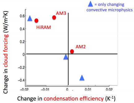 A measure of cloud feedback (vertical axis) plotted against a property of the sub-grid closure for moist convection (horizontal axis) for 3 comprehensive atmospheric models developed at GFDL (red dots) and 3 versions of a prototype of a new atmospheric model, the 3 versions differing only in the treatment of “microphysics” within the sub-grid convective closure (blue triangles). Redrawn from Zhao et al 2016.
The current generation of global atmospheric models in use for climate studies around the world do some things remarkably well, as I’ve tried to argue in several earlier posts. But it is well known that they struggle with a part of the system that is critical for climate sensitivity: simulating the Earth’s cloud cover and how it responds to warming. They also struggle with simulating those aspects of the tropical climate that are sensitive to the moist convection that occurs on small horizontal scales — the effects of this small-scale convection need to be incorporated into climate models with uncertain “sub-grid closures”. Unfortunately, the treatment of moist convection affects cloud feedbacks.
At GFDL we have built a variety of atmospheric models over the past 10-15 years, but they are almost all closely related to 3 distinct models AM2, AM3, and HiRAM. The 3 models differ especially in their sub-grid closures for moist convection. AM3 and HiRAM generate larger positive cloud feedbacks than AM2. We are in the process of trying to construct a new, hopefully improved, atmospheric model (“AM4”) so we are naturally interested in understanding the key distinction between our earlier efforts that resulted in differing cloud feedbacks. This is not straightforward since cloud feedbacks are properties of the model that emerge from the interactions between a number of model components. Ming Zhao took the lead in this detective work, reporting in Zhao 2014 that the different cloud feedbacks among these 3 models were primarily related to effects on the short wave feedback of the assumptions concerning microphysics (the micron and smaller scale physics controlling precipitation processes) in the plume models underlying the sub-grid scheme for moist convection. It was mostly low and mid level clouds in the tropics that mattered as opposed to upper tropospheric cirrus.
When you change one part of a model, like the sub-grid convective microphysics, you often have to change another aspect of the model to retain a top-of-atmosphere (TOA) energy balance sufficiently realistic to justify coupling it to ocean and ice models and using it in climate change studies. The sensitivity of the resulting model is often a consequence of the change in model formulation needed to rebalance the model as well as the original modification motivating the change. A more recent paper (Zhao et al 2016) describes a study with AM4 in which we only change the model’s sub-grid convective microphysics in ways that maintain balance in the TOA energy fluxes, requiring no changes in other aspects of the model. The figure shows the results from simulations from the atmosphere/land model, in which the sea surface temperatures are prescribed at observed values in a control simulation, then raised by 2K (holding CO2 fixed) and then looking at the change in TOA radiative fluxes. The larger the increase in the net flux out of the system in response to the 2K surface warming, the stronger the radiative restoring force and the smaller the climate sensitivity. (This is sometimes referred to as the Cess senstiviity in honor of Bob Cess who proposed this setup to quantify radiative feedbacks in atmospheric models (Cess et al 1989).) Here we isolate the effects of clouds on the Cess sensitivity by computing the change in cloud forcing, which is now often referred to as the cloud radiative effect. As the model is running, we compute the radiative fluxes twice, both with and without clouds, using only the calculation with clouds to interact with the rest of the model. The difference between the TOA fluxes with and without clouds is the cloud forcing — clouds have a net cooling effect on the climate so the cloud forcing is negative. We then repeat this calculation with the +2K perturbation and decompose the change in the net TOA flux into a clear sky part and a part due to the change in the cloud forcing. A positive change in cloud forcing (less negative cloud forcing in the warmer climate) is a warming effect and increases climate sensitivity. (This change in cloud forcing is not quantitatively a good approximation to the cloud feedback in that it does not vanish when “clouds are unchanged” (e.g Soden et al 2004), but the difference is mostly a constant offset so the two are closely correlated. This can be confusing so might be worth returning to some other time.)
The sub-grid convective closure in these models is a source of cloud condensate on the grid-scale. The horizontal axis in the figure is a non-dimensional measure of the efficiency of this process: the amount of condensate produced per unit precipitation. Cloud can also be directly produced in these models on the grid scale — for example, in extratropical storms. Here we are only looking at the cloud produced by the sub-grid closure. After combining these changes in cloud forcing with the clear sky TOA values, the ratio in the (Cess) sensitivity between the low end and high end models here turns out to be about 1.7– a bit more than half of the factor of 3 uncertainty in sensitivity often quoted. These changes in convective condensation efficiency are small, ranging from – 2% to +1% per degree warming, illustrating the power of clouds to change the energy balance and suggestive of the difficulty in constraining this metric with observations..
Why do we need sub-grid convective closures in our climate models? The atmosphere in the tropics is typically conditionally unstable — parcels of air are stable to ascent if unsaturated but are often unstable if lifted beyond the point at which they become saturated. Within a 100km2 grid box, say, there is a lot of sub-grid turmoil that can create unstable parcel ascent in some fraction of the box. If you do not parameterize the effects of this sub-grid creation of buoyant plumes, you have to wait for the grid box to become saturated and then contend with the often violent, unrealistic convection that would occur in the model on the grid scale. For some time I have felt that we should take models with no sub-grid convective closure more seriously; this simplifies the model a lot and it is interesting to isolate what the sub-grid convection scheme is doing to the simulations. There is more effort in this direction recently (e.g. Webb et al 2015) But there is no claim that at typical GCM resolutions we can avoid sub-grid convective parameterization without degrading the quality of the simulation. It seems that we are stuck with this layer of complexity until we adequately resolve the convection itself, or find some trick like superparameterization to get us to these global “cloud resolving” models more quickly (see post #65).
These closure schemes are often based on a picture of plumes in which the upward motion is assumed to be concentrated and that entrain environmental air, precipitate out some water, and detrain vapor and condensate to the grid-scale as they ascend. Assumptions concerning the turbulence controlling the entrainment and detrainment get a lot of attention — you typically find that many aspects of the tropical simulations, not just cloud feedbacks but many aspects of tropical meteorology, are sensitive to these assumptions about the cloud macrophysics. Before beginning this study, based on the previous literature I suspected that these entrainment assumptions were the source of the differences between our models, but that was not the case — it was the microphysical assumptions instead. You need a microphysical picture to decide how much you precipitate and how much condensate (cloud) remains suspended in the atmosphere. The effects on tropical meteorology of these convective microphysical assumptions are more subtle than those concerning cloud macrophysics. but they still affect cloud feedbacks.
In one class of models, the microphysical picture within the convective sub-grid closure effectively provides a threshold condensate density above which precipitation becomes very efficient. As the climate warms, for a given upward mass flux in a plume there is more water vapor and more condensation but a limit to how much condensate you can suspend and carry around. The result is less cloud condensate produced per unit precipitation. HiRAM and AM3 have this threshold flavor, and the simulation marked by the triangle near the top of the figure is configured to behave in this way as well. Alternatively, the microphysical picture might be such as to make the condensate production more or less proportional to the precipitation as temperatures increase, keeping convective precipitation efficiency about the same. AM2 behaves like this as do the models that produce the two lower blue triangles (these differ in the parameter setting within this scheme).
Can we choose between the different blue triangles based on observations? Direct cloud scale observations of these small changes in the condensation efficiency with temperature are difficult. An alternative is to search for indirect constraints based on emergent properties of the simulation (e.g. Klein and Hall 2015). The problem is that, while it may be possible to find some properties of the climate simulation that look better in one of these models than the others, the biases in other parts of the model affecting the same metric can make it hard to make a convincing case that you have constrained cloud feedback. At this point, we are not convinced that we have emergent constraints that clearly favor one version of this proto-AM4 model over the others. We are uncomfortable having the freedom to engineer climate sensitivity to this degree. You can always try to use the magnitude of the warming over the past century itself to constrain cloud feedback, but this gets convolved with estimates of aerosol forcing and internal variability. Ideally we would like to constrain cloud feedbacks in other ways so as to bring these other constraints to bear on the attribution of the observed warming.
[The views expressed on this blog are in no sense official positions of the Geophysical Fluid Dynamics Laboratory, the National Oceanic and Atmospheric Administration, or the Department of Commerce.]
Could GASS help you with this selection problem? They use detailed cloud models to jump the scale gap between observations and climate models. When I was working on cloud measurements they were an influential group, I do not know how well known they are in the climate modelling community.
I would also include precipitation processes in cloud micro-physics. Basically everything that has to do with particles. Macro-physics would be the flow.
Thanks, I neglected to mention comparison with cloud resolving models in limited domains as another approach to constraining sub-grid closures. We try to follow this work closely and there is a body of work aimed at testing sub-grid closures in this way, but designing the best tests is not trivial when deep moist convection is involved. I was hoping a while back that radiative-convective equilibrium — horizontally homogeneous moist convective turbulence — was the simplest setup in which to make this comparison but that turned out to have a lot of surprises (see post #19). But the basic idea of using cloud-resolving models as a middleman confronting the data from field programs on the one hand and gcm formulations on the other is an important one.
“The current generation of global atmospheric models in use for climate studies around the world do some things remarkably well, as I’ve tried to argue in several earlier posts. But it is well known that they struggle with a part of the system that is critical for climate sensitivity: simulating the Earth’s cloud cover and how it responds to warming.”
Taking into account that IPCC considers that the net Global heat storage is about 0.6 W m–2:
“considering a global heat storage of 0.6 W m–2 (imbalance term in Figure 2.11) based on Argo data from 2005 to 2010 (Hansen et al., 2011; Loeb et al., 2012b; Box 3.1).”
– IPCC;AR5;WGI;page 181; 2.3.1 Global Mean Radiation Budget
And:
IPCC considers that the central estimate for current total feedback from clouds is also 0.6 W/m²:
“Based on the preceding synthesis of cloud behaviour, the net radiative feedback due to all cloud types is judged likely to be positive. …. the central (most likely) estimate of the total cloud feedback is taken as the mean from GCMs (+0.6 W m–2 °C–1).”
– WGI; AR5; 7.2.6 Feedback Synthesis; page 592
I do believe that the °C above is about 0,85 °C:
“The globally averaged combined land and ocean surface temperature data as calculated by a linear trend, show a warming of 0.85 [0.65 to 1.06] °C3, over the period 1880 to 2012”
– WGI; AR5; Page 5
I guess this means that the current generation of global atmospheric models in use for climate studies around the world just struggles. And if the climate models do anything remarkably well, it is – remarkable.
Not sure why you are comparing the cloud feedback to the heat uptake. In the notation of Post #4, let’s define the heat uptake efficiency, the heat uptake per unit warming, . Using the numbers that you quote,
  0.7 W/(m2 K). Dividing the total radiative restoring strength
  into the cloud feedback
  and the rest of it
  , then the transient climate response is proportional to
  . So it seems to me that the best point of comparison for the cloud feedback
  is
is  A typical value for
  is about 2 W/(m2 K), so we should be comparing
  with
with  using these numbers.
Thank you for your reply. However, I still arrive at the result that the central estimates for net global warming is of comparable size to the cloud feedback.
In this consideration I will disregard the oceans. I will only consider surface and atmosphere energy balance. I will use the classic one – box model in your post # 4. For variables I will use figures provided in IPCC WGI;AR5, or values deduced from that report. Here we go:
dT/dt = (Q – (Beta*Ts)) / c
dT: Temperature increase over time period increment – dt
Q: 2.3 W/m2 – IPCC central estimate for anthropogenic radiative forcing in 2011
Beta: 1.9 W/m2*K – Feedback parameter deduced from IPCC WGI;AR5;TFE.4, Figure 1
Ts: 0.85 K – Surface temperature in 2011 minus surface temperature in 1750
c: J / kg*K – Heat capacity. (the value is irrelevant in this consideration).
If we consider that the net energy rate ( W = J/s ) warming the earth is 0.6 W/m2
( Ref: IPCC;AR5;WGI;page 181) then:
Q – (Beta*Ts) = 0.6 W/m2
IPCC provides a central estimate for Q = 2.3 W/m2, Hence:
(Beta*Ts) = Q – 0.6 = 2.3 – 0.6 = 1.7 W/m2
I believe ( Beta*Ts ) can be thought about as the net, temperature dependent, radiation to space.
From your post # 4: “The strength of the radiative restoring is determined by the constant Beta, which subsumes all of the radiative feedbacks — water vapor, clouds, snow, sea ice — that attract so much of our attention.”
As I understand it, clouds are reducing the radiation back to space:
«The net feedback from the combined effect of changes in water vapour, and differences between atmospheric and surface warming is extremely likely positive and therefore amplifies changes in climate. The net radiative feedback due to all cloud types combined is likely positive.» IPCC;WGI;AR5; page 16
Hence, As I understand it, (Beta * Ts) = 1.7 W/m2 contains all the surface temperature dependent effects increasing or decreasing the radiation to space. Clouds are decreasing the radiation to space by 0.6 W / m2. Hence without the cloud feedback (Beta*Ts) would have been 1.7 W/m2 + 0.6 W/m2 = 2.3 W/m2. Hence, without cloud feed back, the net radiative feedback to space would be equal to the anthropogenic radiative forcing Q = 2.3 W/m2.
(If I am wrong in placing the cloud feedback in the (Beta * T) element, the cloud feedback would have to be part of the radiative forcing element Q = 2.3 W/m2. In this case, without the cloud effect, the radiative forcing Q would be 2.3 W / m2 – 0.6 W / m2 = 1.7 W / m2 . Hence, without cloud feed back, the net radiative feedback to space would still be equal to the anthropogenic radiative forcing.)
No matter how I look at this, judging from central estimates from the IPCC report for 2011:
Without the cloud feedback effect the anthropogenic radiative forcing on earth system would be equal to the radiative feedback to space. And, the net global warming ( 0.6 W/m2) is equal to the cloud feedback ( 0.6 W/m2).
I lose you right away. If we ignore the oceans, then the relaxation time is so small that you can think of the system as equilibrating with the forcing instantaneously, so
  . The 0.6 W/m2 heat uptake that you are comparing other terms with would go away. We can continue this discussion offline if you like.
Is there a connection here with the Stephens argument that climate models tend to produce clouds in the upper ranges of optical depth, whereas observed clouds are in the lower ranges?
https://klimazwiebel.blogspot.com/2010/07/cloudy-or-sunny-future.html
Isaac, what do you think about the actual paper of Tan et al. ( http://science.sciencemag.org/content/352/6282/224 )
where they claim: “Global satellite observations of cloud thermodynamic phases have enabled us to show that unrealistically low SLFs common to a multitude of GCMs lead to a cloud-phase feedback that is too negative. This has important ramifications for ECS estimates. Should the low-SLF bias be eliminated in GCMs, the most likely range of ECS should shift to higher values.”
The basic content of the paper is fine, although I would have preferred more details about how the model was run (perhaps I missed something in the supplementary materials). Was each of the the control runs in radiative balance before the CO2 was increased and, if so, were SST and sea ice biases affected by retuning the model to get agreement with satellite cloud liquid water/ice ratios? But I was not happy with the claim that you highlighted. Before making any claims about climate sensitivity in nature, I would have liked to have seen historical simulations from pre-industrial to the present with the higher sensitivity model described here. What kind of aerosol forcing would be needed to avoid overshooting the observed warming, and would this amount of aerosol forcing be consistent with the observed spatial structure of the observed warming?
Dear Isaac,
An argument that has been put to me questioning the Zhao et al (2016) finding of no satisfactory observational constraint on the realism of versions of the GFDL model having different condensation efficiency parameter settings, and hence different ECS values. It is that the Rodwell and Palmer (2004) method of running the model in NWP mode and seeing how forecast errors in variables such as night-time minimum temperatures, daytime maximum temperatures and rainfall develop in data assimilation cycles over the first few days would enable the “best” region of the relevant parameter value, and hence of the model ECS, to be identified.
Another scientist has told me they disagree that short term NWP performance would tell one much about whether the ECS of that model version was realistic.
May I ask what your own view is?
I appreciate that even if the Rodwell and Palmer method was informative about the “best” setting of the parameter that affected ECS, that would not necessarily imply that it was informative about the ECS of the real climate system, as the model would have many other imperfections.
Nic,
I am not sure. We are moving towards having the capability to do this kind of testing against short term forecasts more systematically. You don’t know until you try it but my guess is that in this case it will not help much. If precipitation efficiency depends (indirectly) on temperature, and temperature is so tightly wound up with the winds and relative humidity in weather systems, it would be difficult to unravel the effect of temperature holding other things fixed. My impression is that the short-term forecasting constraint helps you when you have something that effects the control climate — including the diurnal cycle, etc — it then can help you isolate the cause of this dependence. But if the effect on the control climate is small, and, in spite of that, the effect on sensitivity is significant, I am not sure focusing on short-term forecasts is going to provide the answer.