

Posted on March 12th, 2016 in Isaac Held's Blog
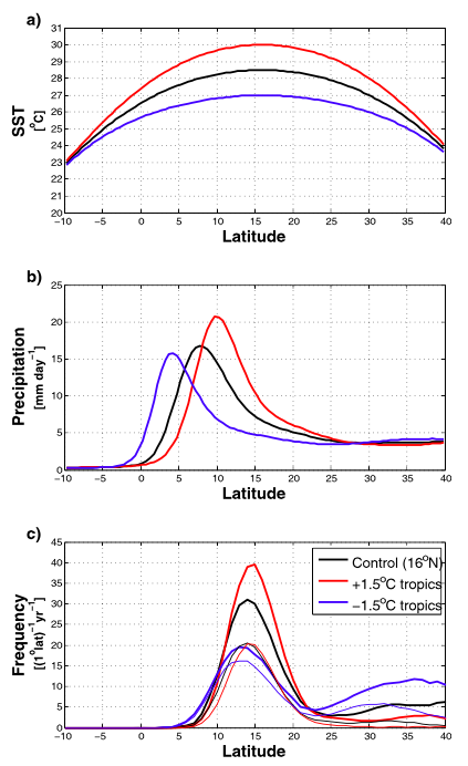 Ttropical cyclone statistics in the global aquaplanet model of Ballinger et al 2015 varying the strength of the surface temperature gradient in the tropics. a) sea surface temperatures; b) precipitation; c) heavy lines: frequency of formation of tropical cyclones; light lines: frequency of formation of tropical cyclones that reach hurricane strength.
There are a lot of open questions regarding how the frequency of tropical cyclones (TCs) is controlled. I’m excited about the fact that our global models are getting progressively better at simulating TC statistics, as I tried to show in post #2. As the quality of global simulations improves it opens up the possibility of manipulating these models in different ways to isolate the factors that alter TC statistics. One approach is to just take a model with realistic boundary conditions (seasonal cycle, continents, orography) and simplify these boundary conditions. A standard simplification is an aquaplanet model in which the surface is uniform and “ocean” covered”, ie water-saturated, typically with no seasonal cycle. With this idealization the model climate, all statistics of the flow — temperatures, precipitation, clouds, radiative fluxes — are functions of latitude (and height) only, and not longitude or time of year, making for a much simpler system to analyze. These aquaplanet simulations are sometimes run with prescribed sea surface temperatures (SSTs) and sometimes with prescribed heat flux through the surface (usually realized by running the atmosphere over a “slab ocean” s saturated surface with some heat capacity, and specifying an “oceanic heat flux” into or out of the slab. With prescribed SSTs, the net energy flux through the surface is part of the solution; in the slab model, the SSTs are part of the solution. I’ve discussed one aquaplanet study of TCs using a slab ocean, Merlis et al 2013, in post #42. We have another paper, Ballinger et al, 2015 using prescribed SSTs. I’ll focus here on the particular result shown above from Ballinger et al. Starting with an SST distribution that is a a function of latitude only and warmer in the Northern than the Southern Hemisphere, we then flatten the SSTs in the tropics as shown in the top panel, keeping the latitude of the maximum SST unmodified (16N in this case). The SSTs outside of the latitudes shown in the figure are also unmodified (this is a global model). Does the number of TCs increase or decrease as the tropical SSTs are flattened?
This particular sensitivity study is of interest in part because some paeloclimates are thought to have had weaker tropical SST gradients. In this paleo context, there have been some arguments that these weak tropical SST gradient climates might have had more tropical storms. Another motivation for looking at this case is the way in which the latitude of the peak tropical rainfall (middle panel) changes when we flatten or sharpen the SSTs. (This maximum is referred to as the ITCZ — the intertropical convergence zone –the north-south flow of the low level air, carrying a lot of water, is converging most strongly at this latitude.) The ITCZ moves northward (towards the maximum in the SSTs) as the SST maximum is sharpened. There is quite a bit of recent literature on the topic of how the ITCZ position is controlled, a lot of it using aquaplanet models (see post #37) This is obviously an important topic, but I won’t try to discuss it here, except to re-emphasize the point that, in this model at least, the latitude of the SST maximum is not in itself determining the ITCZ position.
Quantifying the number of TCs that form in these simulations depends to some extent on the criteria used to identify TCs. The criteria used here are fairly standard: a localized low level vorticity maximum above a threshold, a “warm core”, and near-surface winds of a a given strength lasting for a least a couple of days. Identifying coherent structures of a particular type in fluid flows in not entirely straightforward, but we are pretty confident that the qualitative results don’t depend on the details of these criteria. The thicker lines in the lower panel show the frequency of TC formation as a function of the latitude at which they first satisfy the wind speed criterion. No storms form in the cooler Southern Hemisphere. The latitude at which most of the TCs emerge hardly moves at all as the SSTs are changed in these runs.
The frequency of TC formation decreases as the SSTs are flattened. (There is a secondary mode of formation in the subtropics around 30N; these are vortices that spin off from extratropical frontal circulations penetrating into the subtropics –we did not focus on these in this paper.) The thin lines (a bit hard to see) are the frequency of TC formation counting only those storms that reach hurricane strength at some point in their lifetime. The number of these strong storms does not change much. So the average strength of the TCs increases as the SSTs are flattened. In the flattest case, nearly all TCs reach hurricane strength. As discussed in the paper, these changes are dominated by changes in the SST gradients, not the changes in the tropical temperatures themselves. If you increase the SSTs uniformly the frequency of TC formation decreases in this model, the opposite of the result when you increase tropical SSTs in the manner shown in the figure.
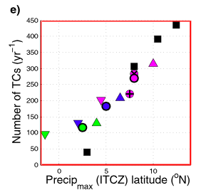
The key to the changes in the number of TCs seems to be closely related to the latitude of the ITCZ, just as in Merlis et al. The following plot from Ballinger et al shows this relationship for the simulations discussed above and also for simulations in which the latitude of the maximum SST and the global mean temperature are changed. The figure also shows the slab ocean results of Merlis et al (black squares). It seems that to understand why the flattening of the SSTs decreases TC numbers in this model we need to understand why the ITCZ moves to lower latitudes. IOt is tempting to think of TCs in this setup as emerging from an instability of the ITCZ, an instability that cannot generate vortices easily when the ITCZ is too close to the equator due to the weakness of the horizontal component of the Coriolis force. The challenge is to translate this picture into a more quantitative theory for the frequency of TC formation. It is interesting that the TC genesis region does not move with the ITCZ; we suspect that this is because the disturbances generated by the instability are just too weak to show up in this metric until they enter the a more favorable region for vortex spin-up. The reason for the increase in average storm intensity with the flattening of SSTs is more obscure but seems related to the fact that storms last longer when the tropical SSTs are relatively flat and so have more time to develop to their mature intensities before migrating to higher latitudes.
 Often a more idealized setup such as this provides a cleaner way of understanding differences between models. It will be interesting to see how robust these kinds of results are across models and how they change as the resolution of the models is improved. These simulations use a 50km grid, which is intuitively far from adequate for tropical cyclone simulations, a point that I am sure would be seconded by most tropical cyclone specialists. (But I place a lot of weight on the result that he version of this 50km model with realistic boundary conditions, counterintuitively perhaps, produces an impressive simulation of TC frequency statistics, as discussed in #2.)
How can this kind of idealized model ever be compared to observations? Among other things, the ITCZ position presumably plays a more important role here than in reality where there are other paths to cyclogenesis not closely tied to a well-defined ITCZ. I think the key is to think of this idealized version as part of a hierarchy that includes the version with realistic boundary conditions. You confront the realistically configured model with observations and use the idealized model to help understand this more comprehensive model and, hopefully, the atmosphere as well, and to cleanly expose the source of differences between attempts at realistic simulation.
[The views expressed on this blog are in no sense official positions of the Geophysical Fluid Dynamics Laboratory, the National Oceanic and Atmospheric Administration, or the Department of Commerce.]
These idealized boundary condition versions of the model can also be confronted with cloud-system resolving simulations (in addition to confronting a comprehensively configured version of the GCM with observations). This approach has come up in your blog posts about convection and clouds, and it’s potentially valuable in the tropical cyclone context as well. There have been several prototype, short integrations of global models with ~4 km horizontal resolution (the recent paper by Bretherton and Khairoutdinov reviews these
http://onlinelibrary.wiley.com/doi/10.1002/2015MS000499/full.
One could take advantage of the zonally symmetric, aquaplanet boundary condition to reduce the zonal dimension of an equatorial -plane domain and save some computational cost.
The only point that I would add is that ideally a high resolution, cloud-system resolving model, used for this kind of simulation would be tested to see if it is capable of simulating realistic statistics of tropical cyclones with realistic boundary conditions.
Thank you very much for the informative blog. I read Ballinger et al. (2015) last year, but this post motivated me to revisit the paper and it led to a very enlightening experience.
When looking at Fig. 2 and Fig. 3 in Ballinger et al. (2015), I noticed that the model can put the ITCZ at similar latitudes but produce very different distributions of TCs (e.g., vs
vs  ;
;  vs
vs  ). Given the clear SST differences on the ITCZ’s north flank, this finding about TC distributions is perhaps not very surprising.
What intrigues me more is whether forcing the model with alternative SST profiles would yield additional interesting results. Maybe with some profiles that resemble the equatorial cold tongue? Presumably this could push the ITCZ but would allow a better control of the SST within . Although the cold-tongue profile is not quite relevant for an aqua planet, it would carry some similarity with the Atlantic and the E Pacific basins.
The idealized simulations in Ballinger et al. (2015) and companion papers are perhaps more relevant to the Earth climate than many would expect. When looking at the variability of Hadley circulation and TC activity, my colleagues and I did find that they have strong connections in both the Atlantic and the E Pacific basins (we had several papers on this topic). The relation for individual basins is robust across re-analyses and HiRAM output, although models could disagree about many details of the ITCZ (e.g., strength, latitude and updraft structure).
I fully agree that understanding the observations needs great simulations of different hierarchies. The work described here is truly fascinating and promising.
Gan — thanks. Aquaplanet simulations with a sharp ITCZ may very well have a fairly direct relevance to those basins, especially the East Pacific and possibly the Atlantic, that have a well-defined ITCZ. Prescribing zonally symmetric SSTs that more closely match the observed latitude variations in these regions would be interesting. How you go about moving away from the zonally symmetric aquaplanets and adding in other factors important for genesis, such as African Easterly Waves, in a systematic controlled way is a challenge. Andrew Ballinger has some aqauplanet simulations with idealized nonzonal (sinusoidal) SSTs in his thesis.
Thank you for the comment. Going beyond the aqua-planet is a natural next step, and I fully agree with your view on the SST and the easterly waves.
Intuitively, the ITCZ (or the meridional overturning circulation) is of the first-order importance for TC activity in the two basins; the seeding by easterly waves probably follows. When looking at the seasonal variability, I saw evidence suggesting that the variability of the oceanic ITCZ and easterly wave activity are connected. A possible explanation is that the Gill-type responses to the ITCZ heating would affect the mean state on which the easterly waves propagate.
That said, the variability of easterly waves is also subject to the impacts of many other factors. In particular, the extratropical influences may be important – as demonstrated by the observational analyses and dry model simulation in Leroux et al. (2011) . If this is indeed the case, getting realistic easterly wave activity would be quite challenging for simple models. (Perhaps surprisingly, the task even turns out very challenging for many realistically configured models, e.g., Martin and Thorncroft (2015) .)
To incorporate easterly waves in idealized models, I probably would start with experimenting with the land, which may help get a more realistic mean flow (esp. in terms of flow instability). Another idea is to introduce some artificial seed generator that mimics the source of easterly waves. It would be interesting to compare the results with the output from the realistically configured HiRAM, which did fairly well in simulating African easterly waves.
Also thanks for guiding me to Andrew’s dissertation. The results of zonally asymmetric SST forcing have many intriguing threads. I haven’t finished the reading yet, but what I saw so far is quite exciting.
I like the idea of adding artificial localized seeds to the aquaplanet, as a simpler step before trying to generate African easterly waves through instabilliy of a low-level easterly jet in an idealized setup. I hadn’t thought about that.
Sorry for reviving an old post. I recently read the dissertation by Erica Staehling and really like the discussion of the co-variability of easterly waves and tropical cyclones. The contradictory results noted in the dissertation used to be confuse me (and likely some other scholars) very much. Maybe a future post can be dedicated to the topic and introduce the results to the community?
Thanks Gan, I have mentioned your interest to Erica. There are a lot of regional issues regarding TC development that can be more and more fruitfully addressed with global models as they continue to improve in their TC simulations. The African easterly wave/TC connection is one of the most interesting.I’ll think about the post you mention — I can’t seem to find the time to post on anything lately, let alone something this intricate.