

Posted on June 3rd, 2016 in Isaac Held's Blog
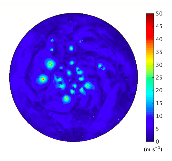
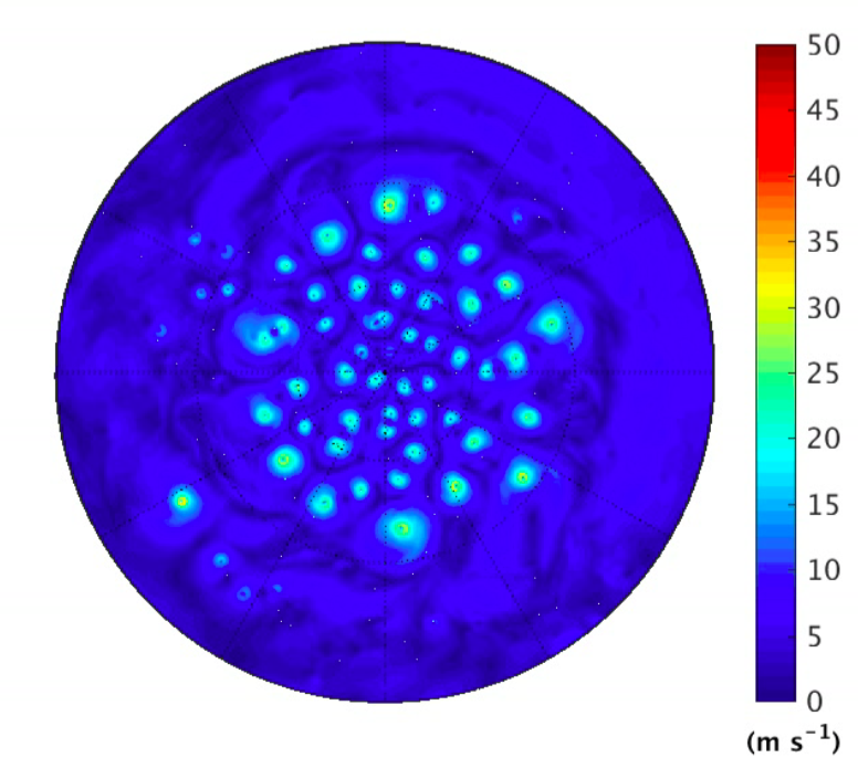 Snapshots of near surface wind speed in simulations of spherical rotating radiative convective equilibrium, as described in Merlis et al 2016. A full hemisphere is shown, the outer boundary being the equator. The surface temperature is prescribed at 307K in the upper panel and 297K in the lower panel. For animations of one month simulations click on (307, 297).
Continuing a recurrent theme in these posts, I’ll describe yet another idealized framework for thinking about the climatology of tropical cyclone (TC) formation. In this setup, we assume a rotating sphere with a homogeneous surface — water-saturated; no continents; surface temperatures prescribed to be uniform over the entire sphere. There are no seasonal or diurnal cycles in the insolation (and we prescribe a spatially uniform ozone distribution as well). So the only source of spatial inhomogeneity is the rotating sphere. For our thin rapidly rotating atmospheric spherical shell, the key inhomogeneity is the latitude dependence of the strength of the horizontal component of the Coriolis force, the “Coriolis parameter”, 


Being spatially inhomogeneous this model is potentially a lot more complicated than the homogeneous model described in Post #43 that uses a a doubly-periodic “
Compared to the more standard aquaplanet simulations described in posts #42 and #67, this setup has the simplification of surface temperatures that are uniform in latitude as well as longitude. When you prescribe more realistic surface temperatures with an equator-to-pole gradient, you get large east-west winds and instabilities resulting in midlatitude storms. These aquaplanet frameworks may be ideal for studying the interactions between TCs and extratropical storms, but it is also nice to get rid of these storms altogether to see how the TC’s behave on their own, which is just what the uniform sea surface temperatures do.
There was some earlier work with more or less this same setup, but focusing on the mean precipitation rather than TC statistics — such as Kirtman and Schneider 2000, who describe a model in which the tropical precipitation still gathers itself into a sharp intertropical convergence zone at the equator despite the absence of any spatial inhomogeneity in the lower boundary condition or the incident solar flux. The theory for this kind of organization of the mean precipitation is itself of interest, but this earlier work did not discuss TC simulation. Tim Merlis, Wenyu Zhou, Ming Zhao and I were discussing this framework — it has the nice feature that anyone with a GCM can configure it easily — but I was personally rather discouraged by the complexity coming from the inhomgeneity of both the mean climate and the TCs. However, more recently Shi and Bretherton 2014 returned to this setup but focusing on TCs, with a lot of interesting results that caught our interest. So we tried our hand at this framework in Merlis et al 2016. We used somewhat higher horizontal resolution (about 50 km) and focused in particular on the response to increasing surface temperatures.
Most importantly from my perspective is that this model and the homogeneous
The figure at the top shows a snapshot (and animations) of the near-surface wind speed for simulations with two different surface temperatures, 297 and 307. The basic picture is of TC genesis in low latitudes , after which the storms migrate poleward and congregate into a swarm of cyclonic vortices around the pole. The situation in the polar cap resembles the
In the colder case, there are obviously a lot more vortices with less space between them, and the crowd of vortices surrounding the pole has grown — to the extent that any more growth could interfere with the generation process in low latitudes. It is not only the number of vortices but the generation rate is also much higher in the case with colder temperature, by roughly a factor of 4. Admittedly, this is a big change in temperature but even when you look at the reduction in genesis frequency per degree warming it is quite a bit larger than the reduction that you see in this model when configured with realistic boundary conditions. (You may recall that the aqua-planet slab ocean model described in Post #42 actually has the frequency of TC formation increasing with increasing surface temperature.)
I think this may be a good setup for looking at how different global model formulations affect TC genesis frequency — and the temperature dependence of this frequency — as long as the 
[The views expressed on this blog are in no sense official positions of the Geophysical Fluid Dynamics Laboratory, the National Oceanic and Atmospheric Administration, or the Department of Commerce.]