

Posted on July 26th, 2011 in Isaac Held's Blog
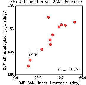
From Son et al 2010, based on the CCMVal ensemble of models, the decorrelation time of the Southern annular mode (SAM) plotted against the simulated latitude of the surface westerlies. Also included is an estimate from NCEP-NCAR reanalysis.
A series of studies over the past decade, starting with Thompson and Solomon 2002, have built a very strong case that the ozone hole in the Southern Hemisphere (SH) stratosphere has caused a poleward shift in the SH surface westerlies and associated eddy fields, especially during the southern summer. The poleward shift is often described as a trend towards a more positive phase of the Southern Annular Mode (SAM). The SAM is a mode of atmospheric internal variability characterized by north-south shifts in the surface westerlies.
The mechanism by which the ozone hole causes this poleward shift is a hot topic in dynamical meteorology. Not only is this response to the ozone hole important in itself, but related mechanisms likely govern the effects on the troposphere of stratospheric perturbations due to volcanic eruptions, the solar cycle, and internal variability. The starting point is the cooling of the lower stratosphere in the vicinity of the ozone hole, due to loss of UV absorption, thereby changing the north-south temperature gradient and associated wind fields in the lower stratosphere. But there are a lot of competing ideas about how altered lower stratospheric winds and temperatures in turn affect the fluxes of angular momentum that maintain the surface westerlies. (Some of my own lectures on the basic dynamics controlling the surface westerlies, including the key role of transport of angular momentum associated with the midlatitude storm tracks, can be found here.) GCMs consistently simulate a poleward shift in response to the ozone hole but of varying magnitude. They also consistently simulate a poleward shift due to increasing CO2.
AR4 was noncommital on the relative importance of greenhouse gases and the ozone hole for the observed SH wind shift. But a number of more recent papers have argued that this shift is primarily a response to ozone depletion, rather than CO2 (see Son et al 2010, Polvani et al 2011). Does this mean that the westerlies will bounce back as the ozone hole heals, assuming that we can continue to avoid emitting CFCs? When models are used to project into the future, this bounce back typically does not occur; the tendency for the winds to return equatorward is compensated, or overcompensated in some models, by the effects of the CO2 increase — the healing is projected to occur more slowly than did the generation of the ozone hole, so the CO2 -induced trend in these models is more competitive with the ozone-induced trend in the future.
But how do we judge the ability of a model to simulate forced shifts in the midlatitude westerlies?. Gerber et al 2010 provide a nice summary of a variety of tests applied to the CCMVal model ensemble to evaluate the realism of the simulated stratosphere-troposphere coupling. I focus here on one specific test, related to the internal variability of the Southern Annular Mode.
Projecting atmospheric variability in observations or models onto the SAM index, one gets a covariance that can be approximated by exponential decay with a decorrelation, or persistence, time in the summer of 15-20 days. But this time scale varies quite a bit from model to model. Plotting the decorrelation time in the CCMVal set of models against the latitude of the mean westerlies as simulated in each model, one gets the very nice result in the figure at the top of the post: models that place the climatological westerlies further equatorward have internal variability with more persistence. Importantly, the decorrelation time of the observed SAM (in reanalyses) and the observed latitude of the westerlies falls nicely on the model ensemble regression line.
One can try to think of the SAM as a damped degree of freedom forced by weather noise 


The magnitude of the perturbation to the annular mode index due to the force, 


with


So the decorrelation time of the SAM index may be one of the most important things to get right if we want to model the circulation responses to the ozone hole and to CO2. As the plot at the top indicates, it seems that if one’s SH summertime westerlies are simulated too far equatorward, this correlation time will be too large, and the response of the SAM to the ozone hole will be too large, holding everything else fixed. Results described in Son et al and by Kidson and Gerber 2010 suggest that this picture does explain some of the spread among model responses, although it is not the whole story.
———————————————————–
added on July 27:
Ed Gerber and Soek-Woo Son kindly sent me the following plot, not in the Son et al paper:
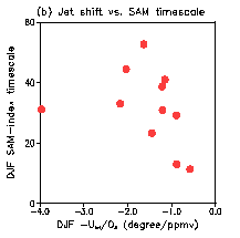
The dots correspond to the CCMval-2 model integrations for the 1980-1999 period. The poleward displacement of the westerly wind maximum (x-axis) is plotted against the SAM time scale. Because O3 is simulated in these chemistry-climate models, responding to changing CFCs in particular, the O3 perturbations differ from model to model, so the displacement is normalized by the O3 perturbation at 50mb averaged over the region polewards of 64S (which assumes that the response to ozone is dominant). The average model displacement, removing this normalization, is about 0.5 degrees/decade. The observed displacement in ERA40 over this time frame is roughly twice as large. Ignoring one outlier, the slope connecting the displacement of the westerlies and the SAM time scale is of the expected sign but somewhat smaller than if the response were simply proportional to

————————————————————–
The CCMVal model ensemble used for the plot at the top of the post is biased, on average, with the latitude of the SH summer westerlies too far equatorward, suggesting that we should reduce the magnitude of the response estimated from the mean of the whole ensemble accordingly. It is interesting that this adjustment happens to takes us in the wrong direction compared to ERA40 trend, which is larger than in most models, so there is still a lot of work to do to figure out exactly what is going on.
It is also interesting that the surface westerlies in SH summer are harder to get right than in any other season/hemisphere, as evidenced by the spread in model results (and personal experience). It also turns out that the annular mode time scale is largest here compared to other seasons and hemispheres. So it is hard to simulate for a good reason — the restoring forces are weak and the westerlies relatively easily perturbed by model errors.
Why is the latitude of the westerlies important for the SAM time scale? This restoring strength is known to be related to the interaction between storm track eddies and the midlatitude jet (see Lorenz and Hartmann 2001). There are a number of recent papers analyzing why this feedback is weaker when the surface westerlies and storm tracks are further polewards. (I find the study of Barnes et al 2010 particularly appealing). One interesting implication of this relationship is that as one pulls the westerlies polewards it should get more and more difficult to pull them even further polewards.
Can one take a similar approach, using the covariance structure of internal variability, to constrain global climate sensitivity? People are pursuing this, and it is certainly worth pursuing. The case of the SAM index and the tropospheric response to the ozone hole is nice in that this response has a structure that is very close to that of the SAM, a dominant mode of internal variability, so the argument that the decorrelation time of this mode is relevant is pretty compelling. The question in the global warming context is whether there are aspects of internal variability that resemble the forced response sufficiently — so we can have confidence that we are looking at the relevant restoring forces.
[The views expressed on this blog are in no sense official positions of the Geophysical Fluid Dynamics Laboratory, the National Oceanic and Atmospheric Administration, or the Department of Commerce.]
Isaac,
This is all very elegant, but what’s the explanation for the CO2-induced poleward shift in the jet? I have seen this produced in models, but I haven’t seen a cogent explanation for the underlying physics.
Also — perhaps not unrelated — every study you cite is about austral summer, but the largest changes in nearly every climate variable in the high southern latitudes (temperature, sea ice, winds..) have been in seasons other than summer. I’ll not hide that I’m being self-interested here, as this something we’ve tried to address (see: Ding et al., 2011).
I’d be interested in your thoughts on both these aspects of the problem.
Warm regards — Eric Steig
Eric, Its pretty clear that the response to ozone is confined to late-Spring-Summer. (I have just started reading the 2010 Ozone Assessment, which has a nice discussion of these things in Ch. 4. As regards to the poleward shift of the westerlies in response to CO2 in GCMs, I don’t think there a fully satisfactory understanding, and it may not be a simple story. I am currently inclined towards those focusing on the different effects of increasing water vapor: increased dry static stability that comes along with more or less constant moist stability; and increased poleward latent energy transport that takes some of the load off mid-latitude eddies, which have to do less sensible transport esp. on the equatorward side of the existing storm-tracks. I will try to post something more coherent on this subject in the near future.
Isaac and Eric,
Ming Cai and I did an idealized coupled simulation for 2xCO2 in which we also found the poleward shift of jet although in the model setting there is no latent heat transport – but there is water vapor feedback in the simulations http://link.springer.com/article/10.1007%2Fs00382-009-0673-x.
In Fig. 4 (f) (convergence of resolved dry static energy transport) of our paper, we did see the decrease in sensible heat transport – only in the lower-troposphere on the equatorial side of storm track, but the total (column-summed, Fig. 4e) sensible heat transport is increased due to the increase in mid-upper troposphere and as a balance to the increase in meridional gradient of net TOA imbalance (Fig 4d). So I am wondering possibly the increase in latent heat transport might not be necessary for the poleward shift of jet.
Jianhua,
There are several studies differing in detail from yours, but similar in that they are dry, which push the westerlies polewards with warming. I am not sure that this is due to the same mechanism that dominates in comprehensive moist GCMs. In these dry models the poleward shift seems to be due to an increase in the meridional temperature gradient near the tropopause — similar to the response to ozone but with the tropopause level temperature gradient increasing due primarily to tropical tropospheric warming rather than lower stratospheric polar cooling. But the observed zonal mean response to the tropical warming associated with El Nino is a contraction of the mid-latitude westerlies equatorwards. If your model can simulate this opposite effect due to El Nino then I would be more confident that it is capturing the relevant mechanisms.
Isaac: Thanks for the suggestion. I’ll have a try on the simulation.
I did not notice the jet shift associated with El Nino until reading your reply. Then I googled and found some interesting papers about the vertical structure of temperatures related to El Nino.
The equatorial shift of westerlies seems to be consistent with El Nino-related vertical-meridional structure of atmospheric temperatures ( Trenberth and Smith, 2009) . The EOF1 in the paper suggests that the upper-tropospheric and stratospheric meridional temperature gradient (between 40N to 90N) associated with El Nino is decreased, contrast to the case in global warming simulations, although in both cases there are zonal-averaged tropical atmospheric warming.
Isaac,
Thank you for posting this.
I have read, and understood as best I can the Gritsun and Branstator paper. As Eric has pointer out this approach is very elegant.
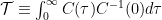
In their section 2 (Theory) they pick over what seems to be a turbulent history of various approaches and attempt to justify their approach but conclude with respect to their Eq 12 (their time varying equivalent to your $latexmathcal{T} equiv int_{0}^{infty} C(tau)C^{-1}(0) dtau$) :
“Consequently, the Kraichnan theorem is not valid, and so it is unclear why one should use (12) as an approximate formula for the system response operator.”
Unclear or not, the strength of the concluding sections dealing with skill and application seem sufficient justification for proceeding whilst awaiting a decision on the desired theoretical justification.
I have previously seen Grant Branstator present this approach in a video recorded at the Isaac Newton Institute here: https://sms.cam.ac.uk/media/872229 and I was fascinated at that time.
That this approach should work at all seems to belie some notions concerning the climate/weather system particularly its ergodic nature, here I refer simply to the convergence of the integrals needed to obtain the sample means and sample response matrices and that they result in demonstrable skill indicating that they may be estimates of actual existing means and response matrices. In my view this is significant not just as a technical achievement but in that it argues against some that might suggest that the notions of mean and covariance are meaningless, that the weather/climate system (or its simulation) is somehow all too chaotic to justify such an approach.
There are many details that I should wish to discuss concerning theirs and your application of FDT, including the importance of unforced simulation runs and highly articificial runs (in their case always January).
Alex