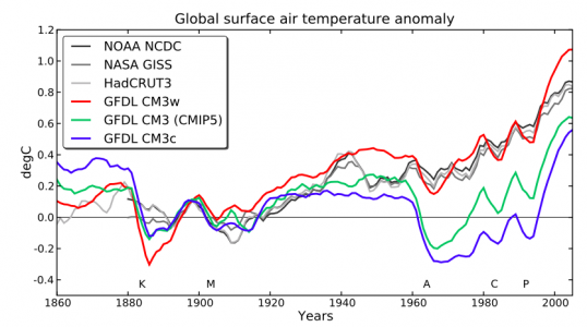
Global mean surface air temperature evolution (with 5-year running mean) in 3 versions of GFDL’s CM3 model (Donner et al, 2011), compared to observations. Each model result is an average over 5 ensemble members. Base period is 1881-1920. From Golaz et al, 2013.
The goal of climate modeling is to develop multi-purpose climate simulators. The same model generating the global mean temperature in this figure is also used to simulate the response of tropospheric winds to the Antarctic stratospheric ozone hole, for example. But as we all know, some aspects of the simulations in our current models are robust while others are sensitive to model uncertainties and may be tunable to some extent within the context of a particular model. If you have a simple model that you are fitting to some data, there is no problem in describing in detail how you decided on the model, the free parameters, the fitting procedure, the data used, etc. it can be more of a challenge to make the development path of a climate simulator fully transparent.
A question that gets a lot of attention is whether you should try to tune your model to be consistent with the evolution of global mean temperatures (GMT) over the past century, or if you should withhold that particular iconic data set during model development, justifying its use as a measure of model quality.
Read the rest of this entry »
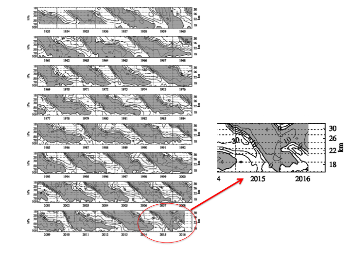
Monthly mean equatorial zonal winds in the stratosphere as a function of time and height. Eastward winds are shaded. 10m/s contour interval. This figure is updated monthly here, thanks to Marcus Kunze. (Original version created by Christian Marquardt (Marquardt, C. (1998): Die tropische QBO und dynamische Prozesse in der Stratosphäre. PhD Thesis, Met. Abh. FU-Berlin, Serie A, Band 9/Heft 4, Verlag Dietrich Reimer Berlin, 260 S.) I have highlighted the last two years.
The quasi-biennial oscillation (QBO) in the equatorial stratosphere is one of the more remarkable phenomena in our atmosphere. In a region of about 15 degrees north and south of the equator, the east-west winds change directions, from about 20 m/s eastward to 30m/s westward and back again with roughly a 27 month period. As seen in the height/time plot shown above, these alternating winds first appear with a given sign at upper levels and then descend more or less regularly before stalling and decaying near the tropopause. There is generally one eastward wind layer and one westward layer at any given time: a new layer of eastward winds appears at upper levels once the previous eastward layer near the tropopause has been squeezed away by descending westward winds. Baldwin et al. 2001 is a classic review of both observational and theoretical aspects of the QBO.
In its most recent evolution, the QBO has exhibited some strange behavior, as seen in the plot shown above — in the past year westward winds unexpectedly appeared at about 40 mb, interrupting the eastward winds in their familiar steady descent. This unusual behavior, evidently with no good analog over the period of our observations of the QBO, is discussed in two recent papers: Newman et al 2016 and Osprey et al 2016.
Read the rest of this entry »
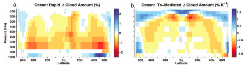
Percent change in zonally-averaged cloud cover over the oceans as a function of latitude and height in response to an instantaneous quadrupling of CO2, decomposed into two parts: (a) a fast adjustment that occurs before surface temperatures have warmed appreciably, and (b) a part that scales linearly with the warming of surface temperature as the system adjusts to the increase in CO2. From Zelinka et al 2013 (as reproduced in Sherwood et al 2015).
The forcing-feedback language used in discussing climate change is familiar but is evolving in interesting directions. I discussed some of the arbitrariness in the decomposition of the feedback into components in posts #24 and #25. (I‘m still serious about discarding the traditional concept of “water vapor feedback” by the way). Here I’ll focus instead on the distinction between forcing and feedback.
In the simplest picture, “forcing” is the result of a radiative transfer calculation that does not depend on the climate response — hold everything else fixed (temperature, water vapor, clouds, etc) and change only the forcing agent (ie CO2); the radiative forcing is the resulting change in flux at the tropopause. But we also speak of “forcing” and “feedback” when emulating GCMs with simple energy balance models. Among other things this helps us isolate the source of differences among GCMs and between GCMs and observations. But these two ideas — forcing as a purely radiative computation, and forcing as a parameter in an emulator of GCM responses — are not fully consistent.
Read the rest of this entry »
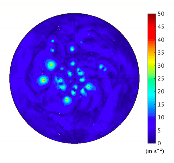
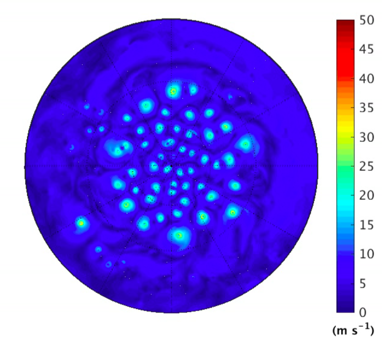 Snapshots of near surface wind speed in simulations of spherical rotating radiative convective equilibrium, as described in Merlis et al 2016. A full hemisphere is shown, the outer boundary being the equator. The surface temperature is prescribed at 307K in the upper panel and 297K in the lower panel. For animations of one month simulations click on (307, 297).
Continuing a recurrent theme in these posts, I’ll describe yet another idealized framework for thinking about the climatology of tropical cyclone (TC) formation. In this setup, we assume a rotating sphere with a homogeneous surface — water-saturated; no continents; surface temperatures prescribed to be uniform over the entire sphere. There are no seasonal or diurnal cycles in the insolation (and we prescribe a spatially uniform ozone distribution as well). So the only source of spatial inhomogeneity is the rotating sphere. For our thin rapidly rotating atmospheric spherical shell, the key inhomogeneity is the latitude dependence of the strength of the horizontal component of the Coriolis force, the “Coriolis parameter”,  where
where  is the latitude. The amplitude of
  increases from the equator, where it vanishes, to the poles. This latitudinal gradient in is critical for TC evolution. In the Northern Hemisphere, the increase of with latitude causes cyclonic vortices to drift north and west with respect to the larger scale flow in which they’re embedded, a process known as
  -drift. ( is the conventional symbol used to represent the northward gradient of .) Read the rest of this entry »
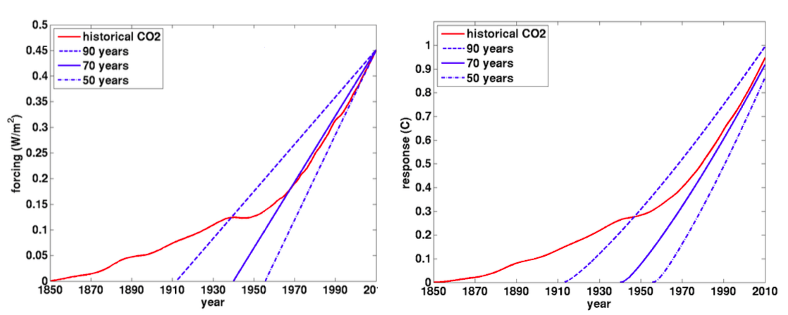
The radative forcing (left) and global mean temperature response (right) using a simple GCM emulator, for the historical CO2 forcing (red) and for the linearly increasing forcing consistent with the simulations used to define the transient climate response (blue), for 3 different ramp-up time scales, the 70 year time scale (solid blue) corresponding to the standard definition.
The terminology surrounding climate sensitivity can be confusing. People talk about equilibrium sensitivity, Charney sensitivity, Earth system sensitivity, effective sensitivity, transient climate response (TCR), etc, making it a challenge to communicate with the public, and sometimes even with ourselves, on this important issue. I am going to focus on the TCR here (yet again). The TCR of a model is determined by what appears to be a rather arbitrary calculation Starting with the climate in equilibrium, increase CO2 at 1% per year until doubling (about 70 years). The global mean warming of the near surface air temperature at the time of doubling is the TCR. In a realistic model with internal variability, you need to do this multiple times and then average to knock down the noise so as to isolate the forced response if you are trying to be precise. If limited to one or two realizations, you average over years 60-80 or use some kind of low-pass filter to help isolate the forced response. Sometimes the TCR is explicitly defined as the warming averaged over years 60-80. Although I have written several posts emphasizing the importance of the TCR in this series, I would like to argue for a de-emphasis of the TCR in favor of another quantity (admittedly very closely related – hence the modesty of this proposal.) Read the rest of this entry »
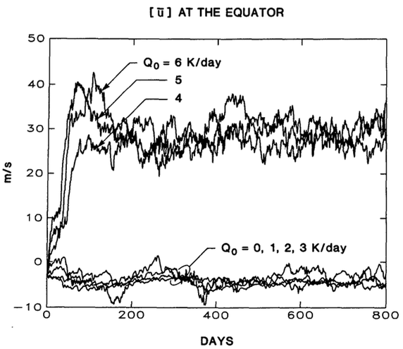
The average around the equator of the eastward wind in the upper tropospheric layer of the idealized atmospheric model of Suarez and Duffy 1992, for several different values of the strength of an imposed tropical heat source.
GCMs often play a conservative role as a counterpoint to speculation or idealized modeling regarding “tipping points” or abrupt climate change, in favor of gradual, more linear climate response to external forcing. Think of abrupt collapse of the AMOC (Atlantic Overturning Circulation) or the “death spiral” of Arctic sea ice. These high-end models may not always be correct of course, but I think they provide an appropriate null hypothesis that must be critically examined in the light of observational constraints, possible missing physics, etc. I’ll use the problem of equatorial superrotation to illustrate this point — also taking this opportunity to introduce this relatively obscure subject.
Read the rest of this entry »
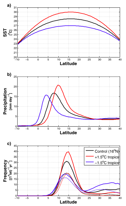
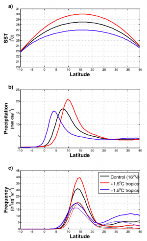 Ttropical cyclone statistics in the global aquaplanet model of Ballinger et al 2015 varying the strength of the surface temperature gradient in the tropics. a) sea surface temperatures; b) precipitation; c) heavy lines: frequency of formation of tropical cyclones; light lines: frequency of formation of tropical cyclones that reach hurricane strength.
There are a lot of open questions regarding how the frequency of tropical cyclones (TCs) is controlled. I’m excited about the fact that our global models are getting progressively better at simulating TC statistics, as I tried to show in post #2. As the quality of global simulations improves it opens up the possibility of manipulating these models in different ways to isolate the factors that alter TC statistics. One approach is to just take a model with realistic boundary conditions (seasonal cycle, continents, orography) and simplify these boundary conditions. A standard simplification is an aquaplanet model in which the surface is uniform and “ocean” covered”, ie water-saturated, typically with no seasonal cycle. With this idealization the model climate, all statistics of the flow — temperatures, precipitation, clouds, radiative fluxes — are functions of latitude (and height) only, and not longitude or time of year, making for a much simpler system to analyze. These aquaplanet simulations are sometimes run with prescribed sea surface temperatures (SSTs) and sometimes with prescribed heat flux through the surface (usually realized by running the atmosphere over a “slab ocean” s saturated surface with some heat capacity, and specifying an “oceanic heat flux” into or out of the slab. With prescribed SSTs, the net energy flux through the surface is part of the solution; in the slab model, the SSTs are part of the solution. I’ve discussed one aquaplanet study of TCs using a slab ocean, Merlis et al 2013, in post #42. We have another paper, Ballinger et al, 2015 using prescribed SSTs. I’ll focus here on the particular result shown above from Ballinger et al. Starting with an SST distribution that is a a function of latitude only and warmer in the Northern than the Southern Hemisphere, we then flatten the SSTs in the tropics as shown in the top panel, keeping the latitude of the maximum SST unmodified (16N in this case). The SSTs outside of the latitudes shown in the figure are also unmodified (this is a global model). Does the number of TCs increase or decrease as the tropical SSTs are flattened? Read the rest of this entry »
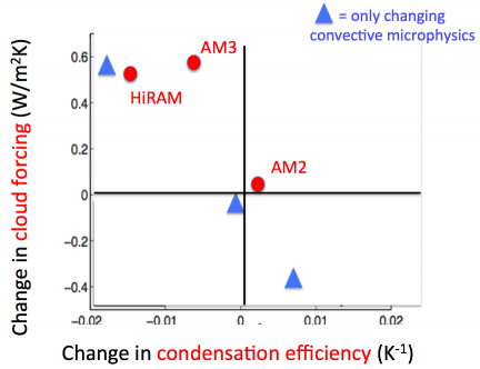 A measure of cloud feedback (vertical axis) plotted against a property of the sub-grid closure for moist convection (horizontal axis) for 3 comprehensive atmospheric models developed at GFDL (red dots) and 3 versions of a prototype of a new atmospheric model, the 3 versions differing only in the treatment of “microphysics” within the sub-grid convective closure (blue triangles). Redrawn from Zhao et al 2016.
The current generation of global atmospheric models in use for climate studies around the world do some things remarkably well, as I’ve tried to argue in several earlier posts. But it is well known that they struggle with a part of the system that is critical for climate sensitivity: simulating the Earth’s cloud cover and how it responds to warming. They also struggle with simulating those aspects of the tropical climate that are sensitive to the moist convection that occurs on small horizontal scales — the effects of this small-scale convection need to be incorporated into climate models with uncertain “sub-grid closures”. Unfortunately, the treatment of moist convection affects cloud feedbacks.
Read the rest of this entry »
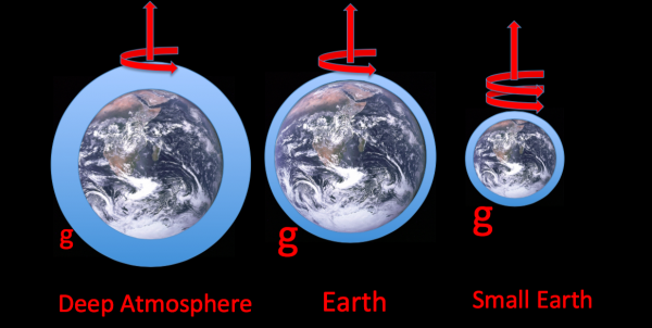
A key problem in atmospheric modeling is the large separation in horizontal scales between the circulations that contain the bulk of the kinetic energy and dominate the horizontal transport of heat, momentum, and moisture, and the much smaller convective eddies that provide much of the vertical transport, especially in the tropics. We talk about the aspect ratio of a flow, the ratio of its characteristic vertical scale to its horizontal scale. The large-scale eddies dominating the horizontal transport have very small aspect ratios. These eddies (extratropical storms and even tropical cyclones) are effectively pancakes. In contrast, the small-scale convective motions have aspect ratios of order one. You have to get the horizontal grid size down well below the vertical scale of the atmosphere — the tropopause height or the scale height — to begin to resolve these small-scale motions. They are not resolved in current global climate models, a fact that colors all of climate modeling. We try to develop theories (closure schemes) for the vertical fluxes by unresolved eddies, but that’s hard and success is limited. So groups around the world are developing global models with horizontal resolution of a few kilometers. (The animation in post #19 is produced by a model of this resolution but in a very small domain a few hundred kilometers on a side.) While these high resolution models don’t resolve all of the vertical transports, global models with horizontal grid size of 1km or so will clearly help a lot. But we are still pretty far from being able to utilize global models with such high resolution as a flexible tool in climate research. They are too slow on available computing resources. So we look for shortcuts.
Read the rest of this entry »
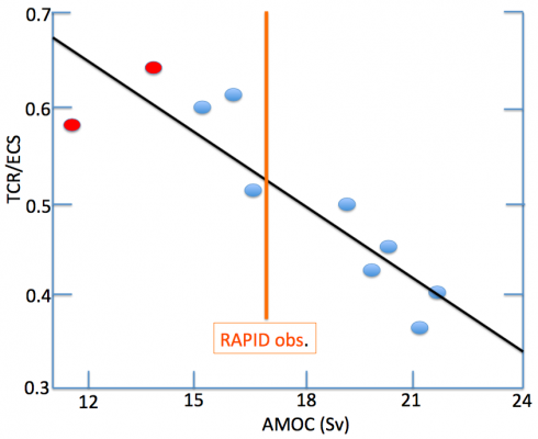
The strength of the Atlantic Meridional Overturning Circulation (AMOC) at 26N , in units of Sverdrups (106 m3/s), plotted against the ratio of the Transient Climate Response to the Equilibrium Climate Sensitivity (TCR/ECS) in a set of coupled atmosphere-ocean climate models developed at GFDL over the past 15 years. Redrawn from Winton et al 2014. Also shown is the strength of the AMOC as observed by the RAPID array at 26N, from McCarthy et al 2015.
An important piece of information about the climate’s response to CO2 (and the other long-lived greenhouse gases) is the degree to which the forced response manages to equilibrate to the CO2 concentration as it increases. Estimates of the degree of disequilibrium affect the attribution of the warming to date as well our ability to anticipate the longer term response to the anthropogenic CO2 pulse. Most of the oceanic heat uptake that determines the degree of disequilibirum occurs either in the Southern Ocean or in the Atlantic Ocean where it is associated with an overturning circulation consisting of less dense waters moving northward near the surface throughout the Atlantic with sinking in the subpolar North Atlantic and a return flow of denser water at depth. I’m focusing here on the latter, the Atlantic Meridional Overturning Circulation, or AMOC. The case for the strength of the AMOC playing an important role in setting the rate of heat uptake by the oceans and the degree of disequilibrium in global mean surface temperature is made in particular by Winton et al 2014 and Kostov et al 2013, who describe two rather different perspectives on why you should expect a relationship between these two quantities.
Read the rest of this entry »


Recent Comments