Isaac Held's Blog

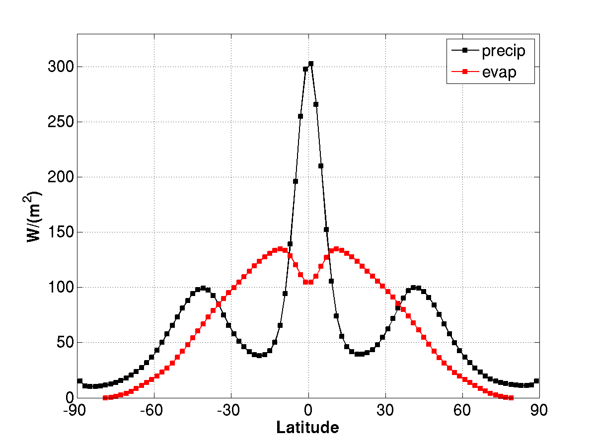
Time-mean precipitation and evaporation as a function of latitude as simulated by an aqua-planet version of an atmospheric GCM (GFDL’s AM2.1) with a homogeneous “slab-ocean” lower boundary (saturated surface with small heat capacity), forced by annual mean insolation.

One often hears the statement the “strength of the hydrological cycle” increases with global warming.  But this phrase seems to mean different things in different contexts.

Read the rest of this entry »

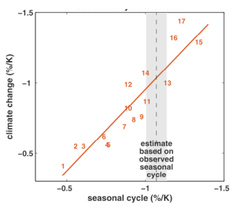From Hall and Qu, 2006.  Each number corresponds to a model in the CMIP3 archive.  Vertical axis is a measure of the strength of surface albedo feedback due to snow cover change over the 21st century (surface albedo change divided by change in surface temperature over land in April).  Horizontal axis is measure of surface albedo feedback over land in seasonal cycle (April to May changes in albedo divided by change in temperature).  The focus is on springtime since this is a period in which albedo feedback tends to be strongest.

There are a lot of uncertainties in how to simulate climate, so, if you ask me,  it is self-evident that we need a variety of climate models. The ensembles of models that we consider are often models that different groups around the world have come up with as their best shots at climate simulation.  Or they might be “perturbed physics” ensembles in which one starts with a given model and perturbs a set of parameters.  The latter provides a much more systematic approach to parametric uncertainty, while the former give us an impression of structural uncertainty— ie, these models often don’t even agree on what the parameters are.  The spread of model responses is useful as input into attempts at characterizing uncertainty, but I want to focus here, not on characterizing uncertainty, but on reducing it.

Read the rest of this entry »

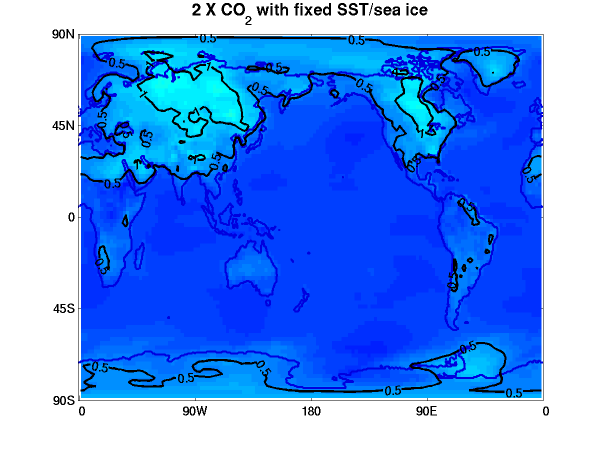
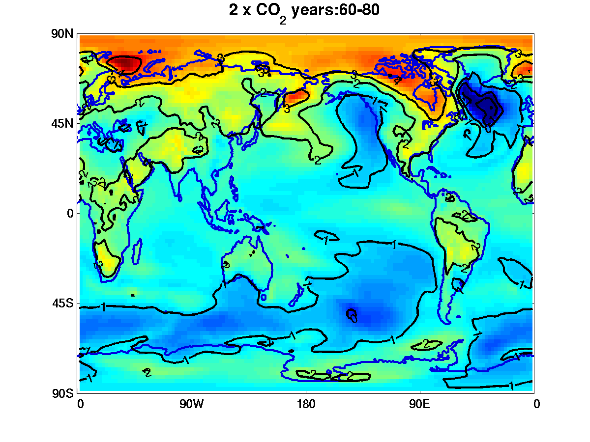
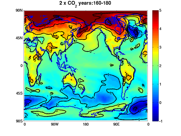
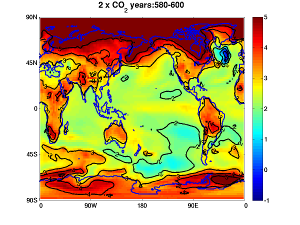
Annual mean surface air temperature response to a doubling of CO₂.  Upper left: equilibrated atmosphere/land response (GFDL AM2.1/LM2.1) with fixed seasonally varying sea surface temperatures (SSTs) and sea ice. Other plots are coupled model (CM2.1) responses in a single realization with CO₂ increasing at 1%/year till doubling (year 70) then held fixed.  Upper right — average over years 60-80, around the time of doubling; lower left — years 160-180; lower right — years 580-600.  Contour interval is 0.5C in upper left and 1C elsewhere.  Colors same in all plots.

Returning to our discussion of the time scales of the climatic response, it might be useful to take a closer look at the evolution of the warming in a GCM for the standard idealized scenario in which, starting from an equilibrated state, CO₂ is increased at 1% per year until it doubles and is then held fixed.  This plot shows the results from our CM2.1 model.

I want to focus especially on the upper left panel; the other panels are mainly included here to provide context. The upper left panel is not generated from the fully coupled model, but from the atmosphere/land components of this model in isolation, holding the sea surface temperature (SST) and sea ice distribution fixed at their unperturbed climatological seasonal cycles, while doubling the CO₂.   This model equilibrates to a change in CO₂ in a couple of months (there is no interactive vegetation or even permafrost in this model, both of which would create the potential for longer time scales regionally).  The response depends on the season, so one has to integrate for at least a year before this annual mean pattern emerges.  We might call this the ultra-fast response, distinguishing it from fast (oceanic mixed layer), slow (oceanic interior), and ultra-slow (anything slower than the thermal adjustment time of the interior ocean, such as aspects of glacier dynamics).  One can visualize this as the first step in the response, but one that is evidently dramatically modified over time by the ocean warming and sea ice retreat.

Read the rest of this entry »

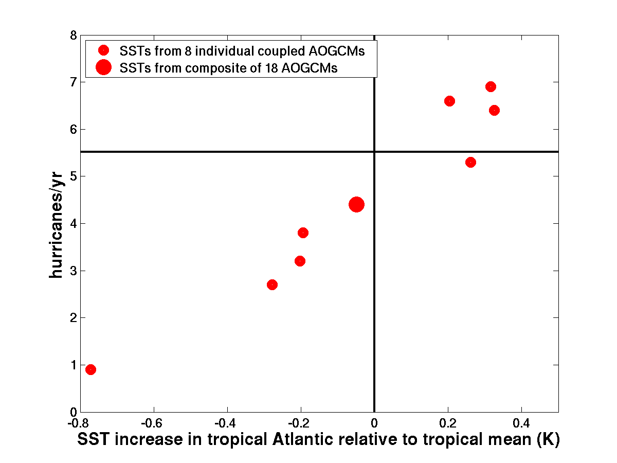
The number of Atlantic hurricanes simulated by the model of Zhao et al 2009, when boundary conditions are altered to correspond to the changes in sea surface temperature (SST) simulated in 8 of the CMIP3/AR4 models for the A1B scenario by the end of the 21st century (small red dots), and to the ensemble mean of the changes in SST in 18 CMIP3/AR4 models (big red dot).  The horizontal line indicates the number of hurricanes/yr  in the control simulation.

These results, and the discussion that follows, are based on collaborative work with Ming Zhao, Gabriel Vecchi, Tom Knutson and other GFDL colleagues. (Some of the model runs utilized here were discussed in  Zhao et al 2009 and Vecchi et al 2011, — the full set will be discussed in a forthcoming paper.)

Given the global atmospheric/land model described in post #2, which appears to simulate certain aspects of the statistics of tropical cyclones in the Atlantic quite well, what does the model predict for the change in these statistics in the future?  And how seriously should we take the result?

Read the rest of this entry »

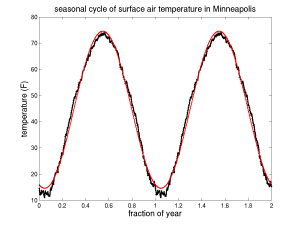
Black: Climatological seasonal cycle of temperature in Minneapolis  (two years are shown for clarity).  Averaging (T_max +T_min)/2 over >100 years for each calendar day.  Data kindly provided by Charles Fisk.  Red: Fit with annual mean plus fundamental annual harmonic

Two common questions that I (and many others) often get are “How can you predict anything about  the state of the atmosphere 100 years from now when you can’t predict the weather 10 days in advance?” and “How do you know that the climate system isn’t far more complicated than you realize or can possibly model?”  I often start my answer in both cases with the title of this post.  It may sound like I am being facetious, but I’m not; the fact that summer is warmer than winter is an excellent starting point when addressing both of these questions.

Read the rest of this entry »

Evolution of global mean near-surface air temperature in GFDL’s CM2.1 climate model in simulations designed to separate the fast and slow components of the climate response in simulations of future climate change, as described in Held et al, 2010.

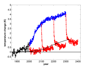
Continuing our discussion of transient climate responses, I want to introduce a simple way of probing the relative importance of fast and slow responses in a climate model, by defining the recalcitrant component of global warming, effectively the surface manifestation of changes in the state of the deep ocean.

The black curve in this figure is the evolution of global mean surface air temperature  in a simulation of the 1860-2000 period produced by our CM2.1 model, forced  primarily by changing the well-mixed greenhouse gases, aerosols, and volcanoes.  Everything is an anomaly from a control simulation.  (This model does not predict the CO₂ or aerosol concentrations from emissions, but simply prescribes these concentrations as a function of time.) The blue curve picks up from this run, using the SRES A1B scenario for the forcing agents until 2100 and then holds these fixed after 2100.  In particular, CO₂ is assumed to approximately double over the 21st century, and the concentration  reached at 2100 (about 720ppm) is held fixed thereafter.  The red curves are the result of abruptly returning to pre-industrial (1860) forcing at different times (2000, 2100, 2200, 2300) and then integrating for 100 years.  The thin black line connects the temperatures from these four runs averaged over years 10-30 after the abrupt turn-off of the radiative forcing.

Read the rest of this entry »

Upper panel: Interdecadal component of annual mean temperature changes relative to 1890–1909. Lower panel: Area-mean (22.5°S to 67.5°N) temperature change (black) and its interdecadal component (red).  Based on the methodology in Schneider and Held, 2001 and HadCRUT3v temperatures.  More info about the figure.

Perhaps the first thing one notices when exposed to discussions of climate change is how much emphasis is placed on a single time series, the globally averaged surface temperature. This is more the case in popular and semi-popular discussions than in the scientific literature itself, but even in the latter it still plays a significant role.  Why such an emphasis on the global mean?

Two of the most common explanations involve 1) the connection between the global mean surface temperature and the energy balance of the Earth, and 2) the reduction in noise that results from global averaging.  I’ll consider each of these rationales in turn. Read the rest of this entry »

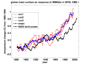Global mean surface air warming due to well-mixed greenhouse gases in isolation, in 20th century simulations with GFDL’s CM2.1 climate model, smoothed with a 5yr running mean

“It is likely that increases in greenhouse gas concentrations alone would have caused more warming than observed because volcanic and anthropogenic aerosols have offset some warming that would otherwise have taken place.” (AR4 WG1 Summary for Policymakers).

One way of dividing up the factors that are thought to have played some role in forcing climate change over the 20th century is into 1) the well-mixed greenhouse gases (WMGGs: essentially carbon dioxide, methane, nitrous oxide, and the chlorofluorocarbons) and 2) everything else.  The WMGGs are well-mixed in the atmosphere because they are long-lived, so they are often referred to as the long-lived greenhouse gases (LLGGs).  Well-mixed in this context means that we can typically describe their atmospheric concentrations well enough, if we are interested in their effect on climate, with one number for each gas.  These concentrations are not exactly uniform, of course, and studying the departure from uniformity is one of the keys to understanding sources and sinks.

We know the difference in these concentrations from pre-industrial times to the present from ice cores and modern measurements, we know their radiative properties very well, and they affect the troposphere is similar ways.  So it makes sense to lump them together for starters, as one way of cutting through the complexity of multiple forcing agents.

Read the rest of this entry »

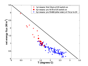The co-evolution of the global mean surface air temperature (T) and the net energy flux at the top of the atmosphere, in simulations of the response to a doubling of  CO₂ with GFDL’s CM2.1 model.
Slightly modified from Winton et al (2010).

Global climate models typically predict transient climate responses that are difficult to reconcile with the simplest energy balance models designed to mimic the GCMs’ climate sensitivity and rate of heat uptake.  This figure helps define the problem.

Take your favorite climate model, instantaneously double the concentration of in the atmosphere, and watch the model return to equilibrium. I am thinking here of coupled atmosphere-ocean models of the physical climate system in which is an input, not models in which emissions are prescribed and the evolution of atmospheric is itself part of the model output.

Now plot the globally-averaged energy imbalance at the top of the atmosphere versus the globally-averaged surface temperature .  In the most common simple energy balance models we would have where both , the radiative forcing,  and , the strength of the radiative restoring, are constants.  The result would be a straight line in the plane, connecting with as indicated in the figure above.  The particular two-box model discussed in post #4 would also evolve along this linear trajectory; the different way in which the heat uptake is modeled in that case just modifies how fast the model moves along the line.

The figure at the top shows the behavior of GFDL’s CM2.1 model.  The departure from linearity, with the model falling below the expected line, is common if not quite universal among GCMs, and has been discussed by Williams et al (2008) and Winton et al (2010) recently — these papers cite some earlier discussions of this issue as well.  Our CM2.1 model has about as large a departure from linearity as any GCM that we are aware of, which is one reason why we got interested in this issue. Read the rest of this entry »

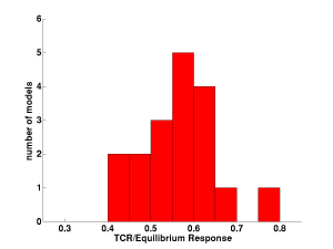Histogram of the ratio of transient climate response (TCR) to equilibrium climate sensitivity in the 18 models for which both values are provided in Ch. 8 of the WG1/AR4/IPCC report

I find the following simple two degree-of-freedom linear model useful when thinking about transient climate responses:

and are meant to represent the perturbations to the global mean surface temperature and deep ocean temperature resulting from the radiative forcing .  The strength of the radiative restoring is determined by the constant , which subsumes all of the radiative feedbacks — water vapor, clouds, snow, sea ice — that attract so much of our attention.  The exchange of energy with the deep ocean is assumed to be proportional to the difference in the temperature perturbations between the surface and the deep layers, with constant of proportionality .  The fast time scale is set by , representing the heat capacity of the well-mixed surface layer, perhaps 50-100m deep on average (the atmosphere’s heat capacity is negligible in comparison), while crudely represents an effective heat capacity of the rest of the ocean. Despite the fact that it seems to ignore everything that we know about oceanic mixing and subduction of surface waters into the deep ocean, I think this model gets you thinking about the right questions. Read the rest of this entry »