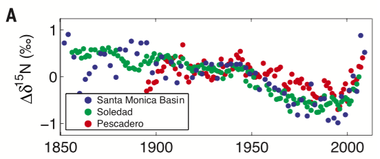
A proxy for the strength of the trade winds in the North Pacific: nitrogen isotope records from three sediment cores off the west coast of North America (blue = 33oN, green =25oN , red = 24oN). More 15N is interpreted as stronger trades. From Deutsch et al. 2014.
The warming of the globe over the last couple of decades has been slower than the forced warming predicted by most GCMs, due to some combination of internal variability, incorrectly simulated climate responses to the changes in forcing agents, and incorrect assumptions about the forcing agents themselves. A number of studies have implicated the tropical Pacific as playing a central role in this discrepancy, specifically a la Nina-like trend — with eastern equatorial Pacific cooling and strengthening trade winds. If you intervene in a climate model by imposing the observed near-surface ocean temperatures in the eastern equatorial Pacific (Kosaka and Xie, 2013) or by imposing the observed surface equatorial Pacific wind fields (England et al 2014; Delworth et al 2015), the rest of the simulation falls into place– not just the global mean temperatures but the spatial pattern of temperature trends over the past two decades — as well as the California drought. The wind and ocean surface temperatures are tightly coupled on annual and longer time scales in this region, so these different studies tell a consistent story. The implication is that explanations for the discrepancy in global warming rate need to simultaneously explain this La Nina-like trend to be convincing. Based on its importance in recent decades, it is tempting to assume that the tropical Pacific has played an important role in modulating the rate of global warming throughout the 20th century. But if the nitrogen isotope record on the eastern margins of the subtropical north Pacific provided byDeutsch et al. 2014and shown above is a good proxy for trade wind strength, it is interesting that it isn’t dominated by quasi-periodic multi-decadal variability. Instead it looks like a long term trend towards weaker trades until the last 20 years or so — a trend that happens to be roughly consistent with the forced response of the tropical winds to greenhouse warming in most models — which is then interrupted by an event that is unique in the context of the last 150 years. (This is admittedly less clear for the red record in the figure than for the green and blue.) Read the rest of this entry »
Upper panel: annual mean northward atmospheric energy transport as a function of latitude averaged over the control simulations in CMIP3. The total flux is shown as well as the decomposition into the latent flux and the dry static energy flux. Lower panel: Response of these fluxes to doubled CO2 (2 x CO2 minus control) in slab-ocean models with fixed oceanic heat transport. Fluxes in petawatts. Courtesy of Yen-Ting Hwang.
A warming atmosphere typically results in larger horizontal moisture transports. In addition to the implications for the hydrological cycle and oceanic salinity discussed in previous posts, this increased moisture transport also has implications for energy transport. If energy is used to evaporate water at point A and the vapor is transported to point B where it condenses, releasing the heat of condensation, energy has been transported from A to B. This latent heat transport is a large component of the total atmospheric energy transport. The thin dotted line in the top panel above is the northward latent heat transport averaged across the CMIP3 models. Outside of the tropics, eddies are mixing water vapor downgradient, resulting in a poleward transport. Close to the equator, the Hadley circulation dominates, with its equatorward flow near the surface that carries water vapor from the subtropics to the tropical rain belts (the compensating poleward flow near the tropopause carries very little water vapor in comparison). This tropical branch with equatorward vapor transport is clearer in the Southern Hemisphere in this plot, due I think to more continents and larger seasonal cycle of tropical rainfall in the north, producing less separation in the annual mean between the tropical and midlatitude rainbelts.
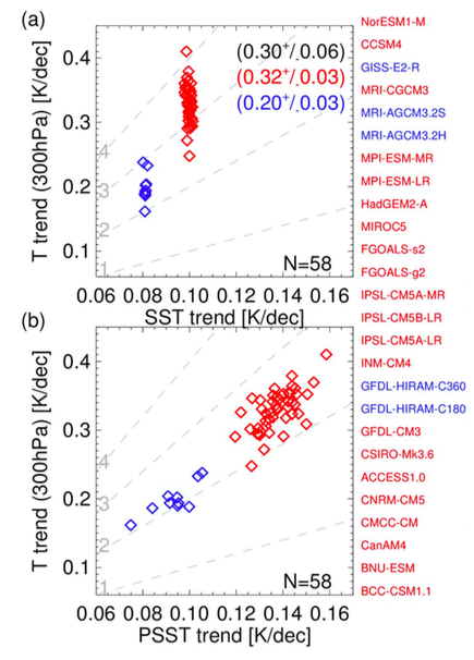
Upper tropospheric warming trends in AMIP (prescribed sea surface temperature) simulations at 300mb over the period 1984-2008 averaged from 20S-20N, in the CMIP5 archive. Red and blue correspond to models that used two different SST data sets. SST on the x-axis in the upper panel is the mean SST over the tropical oceans. PSST in the lower panel is the mean of SST over the tropical oceans weighted by the pattern of precipitation simulated in each model.
Let’s turn once again to the problem of the vertical structure of warming trends in the tropical troposphere. (Warning: this post contains no comparison with data — the point is to try to clarify how to think about the GCM simulations.) In two recent posts, #54 and #55, I discussed a paper, Flannaghan et al 2014, in which my colleagues and I focused on the simulations in the CMIP archives in which sea surface temperatures (SSTs) are prescribed following observations (“AMIP” simulations). There is interesting spread in the upper tropospheric warming trends even in these AMIP simulations, as indicated in the figure above, taken from a new paper Fueglistaler et al 2015. Each dot corresponds to an AMIP run from a different model. In the upper panel, the 300mb temperature trends are plotted against the trends in the prescribed tropical SSTs.
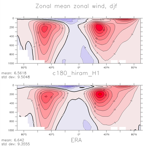
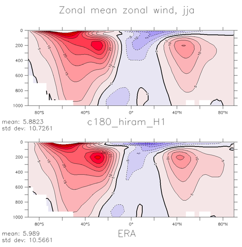
Given the problems that our global climate models have in simulating the global mean energy balance of the Earth, some readers may have a hard time understanding why many of us in climate science devote so much attention to these models. A big part of the explanation is the quality of the large-scale atmospheric circulation that they provide. To my mind this is without doubt one of the great triumphs of computer simulation in all of science.
The figure above is meant to give you a feeling for this quality. It shows the zonal (eastward) component of the wind as a function of latitude and pressure, averaged in time and around latitude circles. This is an atmosphere/land model running over observed ocean temperatures with roughly 50km horizontal resolution. The model results at the top (dec-jan-feb on the left and june-july-aug on the right) are compared with the observational estimate below them. The observations are provided by a reanalysis product(more on reanalysis below). The contour interval is 5m/s; westerlies (eastward flow) are red, easterlies are blue. Features of interest are the location of the transition from westerlies to easterlies at the surface in the subtropics, and the relative positions of the the subtropical jet at 200mb, the lower tropospheric westerlies and the polar stratospheric jet in winter (the latter is barely visible near the upper boundary of the plot when using pressure as a vertical coordinate).
Fig. 9.8 from the AR5 Working Group 1 IPCC report. Global mean surface temperatures simulated by a set of climate models, shown as anomalies from the time mean over a reference period 1961-1990. Observations (HADCRUT4) in black; ensemble mean in red. On the right (circled) are the mean temperatures in the reference period.
Ch.9 of the AR5-WG1 report, “Evaluating Climate Models” is, in my opinion, the most difficult to write of any chapter in that report. You can think of hundreds if not thousands of interesting ways of comparing modern climate models to observations, but which of these is the most relevant for judging the quality of a projection for a particular aspect of climate change over the next century? This is an important research problem. Consider this figure, which shows the familiar simulated changes in global mean surface temperature over the past 150 years, in a set of models deposited in the CMIP5 archive, as anomalies from the model’s own temperature during some reference period (shaded). But the figure also shows in the narrow panel on the right side, circled in red, the models’ mean temperatures during that reference period. People tend to be disappointed when they see this — some models are better than others but the biases in the model’s global mean temperature are typically comparable to the 20th century warming and in some cases larger. If we are interested in projections of global mean warming over the coming century, or in the attribution of this past warming, should we trust these models at all, given these biases?
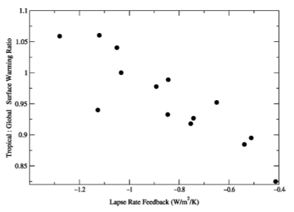
Traditional “lapse rate feedback” in CMIP3 models, over the 21st century in the A1B scenario, plotted against the degree of polar amplification of surface warming in those models (tropical – 30S-30N divided by global mean warming). From Soden and Held 2006.
“Everything should be made as simple as possible, but not simpler.” There is evidently no record of Einstein having actually used these words , and a quote of his that may be the source of this aphorism has a somewhat different resonance to my ear. In any case, I want to argue here that thinking about the global mean temperature in isolation or working with simple globally averaged box models that ignore the spatial structure of the response is very often “too simple”. I am reiterating some points made in earlier posts, especially #5, #7, and #44, but maybe it is useful to gather these together for emphasis.
This animation is the response of a two-dimensional flow on the surface of a rotating sphere to a source that mimics stationary localized heating centered on the equator. The top panel is a north-south component of the wind — red is northward and blue southward. The bottom panel is the streamfunction of the flow –lines of constant streamfunction are the trajectories of fluid particles once the flow becomes steady. At the start of the animation the flow is purely zonal and the forcing is turned on instantaneously and then maintained. The loop covers about 40 days, but the pattern is fully set up in less than half that time. The continental outlines are just meant to help orient the viewer; the surface in this model is featureless. The setup is a classical one for generating a stationary Rossby wave propagating from the tropics into midlatitudes described by Brian Hoskins and colleagues in the late 1970’s and early 80’s (Hoskins et al 1977; Hoskins and Karoly 1981). This kind of wave is the essence of the teleconnections that atmospheric scientists talk about so frequently — patterns of flow that connect widely separated regions. Sometimes the correlations introduced into climate time series by these remotely forced responses can seem like spooky action-at-a-distance. But nothing could be further from the truth. They are just Rossby waves at heart.
Multi-model median of changes in near surface a) temperature, b) relative humidity, and c) equivalent potential temperature between the historical simulation (1975-2004) and the RCP8.5 (2079-2099) simulations in CMIP5. From Byrne and O’Gorman 2013.
In global warming simulations the surface air over land warms more than over the oceans in the tropics, while the relative humidity decreases over land, increasing a bit over the oceans, as illustrated in panels a) and b) above from a recent paper by Michael Byrne and Paul O’Gorman. A quantity that is relevant for the convective instability of the atmosphere and the profile of temperature on a rising air parcel is the equivalent potential temperature, . Strikingly the increase in is quite uniform in the deep tropics, irrespective of whether the underlying surface is land or ocean. This is not an accident and provides us with a simple way of thinking about increasing heat stress with warming.
Vertical profile of temperature trends averaged over 20S-20N in two models. Solid: trends in a 30-year (1970-2000) realization of the CM2.1 coupled model using estimated forcing agents from 1970-2000. Dashed: simulation using the atmosphere/land component of CM2.1 with the same forcing agents but running over the sea surface temperatures generated in this realization of the coupled model.
The previous post summarizes the results from a recent paper, Flannaghan et al 2014, that uses atmosphere/land models running over observed sea surface temperatures (SSTs) to look at the consistency between these models and observations of tropical tropospheric temperature trends. The idea of using this kind of uncoupled model is to try to put aside the issue of SST trends in the tropics and focus more sharply on the vertical structure of the temperature trends. Because models are so consistent in producing a warming trend that is top-heavy in the tropical troposphere, due to the strong tendency to follow a moist adiabatic profile, and because this pattern of change has numerous ramifications for tropical climate more generally, any possibility that this warming profile is wrong takes precedence over other issues in tropical climate change, in my view. I interpret the results in Flannaghan et al to say that microwave sounding data, at least, does not require us to reject the hypothesis provided by climate models for the vertical profile of the tropical temperature trends.
To follow up on the last post, I would like to discuss, or at least mention, some other issues regarding this setup, in which SSTs are simply prescribed as a boundary condition. Could there be something fundamentally flawed about this approach? This may seem like a technical issue, but a large fraction of atmospheric model development takes place in this prescribed SST framework to try to separate biases due to atmospheric model imperfections from those due to the ocean/sea ice model, so it is important to understand its limitations. I have used this kind of setup in a number of posts to address other issues, for example #2,#10, #11, #32, #34; any limitations to this decoupled framework could affect my own thinking about a variety of climate change issues.
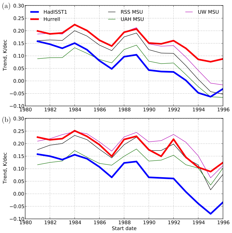
Mid-tropospheric temperature trends (TTT channel — see below) from a given start date till 2008, plotted as a function of start date, in three analyses of the MSU data (thin lines) and in an atmosphere/land model running over two estimates of observed sea surface temperatures: HadISST1 (blue), Hurrell (red). The upper panel is the trend from ordinary least squares while the lower panel uses the Theil-Sen estimator.
In a paper just published, Flannaghan et al 2014, my colleagues (Tom Flannaghan, Stephan Fueglistaler, Stephen Po-Chedley, Bruce Wyman, and Ming Zhao) and I have returned to the question of tropical tropospheric warming in models and observations — Microwave Sounding Unit (MSU) observations specifically. This work was motivated in part (in my mind at least) by the material in Post #21, but the results have evolved significantly. All the figures in this post are from the Flannaghan et al paper.
There are important discrepancies between models and observations regarding tropical tropospheric temperature trends. It is informative if we can divide these into two parts, one associated with the sea surface temperature (SST) trends and the other with the vertical structure of the trends in the atmosphere and how these trends are related to the SST trends. The former is associated with issues of climate sensitivity and internal variability; the latter is related to the internal dynamics of the atmosphere, especially the extent to which the vertical structure of the temperature profile is controlled by the moist adiabat. A moist adiabatic temperature profile is what you get by raising a parcel which then cools adiabatically due to expansion, with part of this cooling offset by the warming due to the latent heat released when the water vapor in the parcel condenses. The tropical atmosphere is observed to lie close to this profile, as do our models. Models continue to approximately follow this profile as they warm., so they invariably produce larger warming in the upper troposphere than at the surface in the tropics — simply because the water vapor in the parcel increases with warming, so there is more heating due to condensation as the parcel rises. All models do this, from global models to idealized “cloud resolving” models with much finer resolution — see Post #20 for a discussion of the latter. The same top-heaviness is seen in the tropospheric temperature changes accompanying ENSO variability, which models simulate very well. Why should lower frequency trends behave any differently than the year-to-year variability resulting from ENSO? If models have this wrong it has a lot of implications.


 A proxy for the strength of the trade winds in the North Pacific: nitrogen isotope records from three sediment cores off the west coast of North America (blue = 33oN, green =25oN , red = 24oN). More 15N is interpreted as stronger trades. From Deutsch et al. 2014.
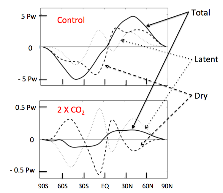


 . Strikingly the increase in
Recent Comments