Animation of near-surface wind speeds in rotating radiative-convection equilibrium, following Zhou et al, 2014.
I have discussed models of non-rotating radiative-convective equilibrium (RCE) in previous posts. Given an atmospheric model one idealizes it by throwing out the spherical geometry, land-ocean configuration and rotation, creating a doubly-periodic planar geometry re-entrant in both x and y, while also removing any horizontal inhomogeneities in the forcing and boundary conditions. In the simplest case, surface temperatures are specified and the surface is assumed to be water-saturated. The result is an interesting idealized explicitly fluid dynamical system for studying how the climate — especially that of the tropical atmosphere — is maintained by a balance between destabilization through radiative fluxes and stabilization through turbulent moist convection. There is a lot that we don’t understand about this setup, which still contains all of the complexity of latent heat release and cloud formation. But even though we don’t understand the non-rotating case very well, it is interesting to re-introduce rotation while maintaining horizontal homogeneity. Adding rotation has a profound influence on the results — the model atmosphere fills up with tropical cyclones! Some colleagues suggest referring to this system as TC World; otherssuggest Diabatic Ekman Turbulence. I’m going to stick with Rotating Radiative-Convective Equilibrium, or Rotating RCE for short.
Zonal (east-west) wind in the lower troposphere (850mb) in two simulations with a 50km resolution atmospheric model with zonally symmetric boundary conditions. Only of longitude within the tropics (30S-30N) is shown. The ITCZ is located at in the upper panel and in the lower panel. Simulations described in Merlis et al 2013. (White, Black) => winds from the (west, east). 6 frames/day for 100 days.
The frequency of formation of hurricanes/typhoons has mostly been studied in the past by trying to develop “genesis indices” – empirical relations between the frequency of storm genesis and the larger scale circulation and thermodynamic structure of the atmosphere. But there is an ongoing transition, picking up steam in a number of atmospheric modeling groups around the world, to using global atmospheric models that simulate hurricanes directly to study how genesis is controlled. One goal of this work is to understand how hurricane frequency responds to the warming resulting from increasing greenhouse gases. Posts #2, 10, and 33 describe some of our recent efforts at GFDL along these lines. That work uses models in a comprehensive setting, with a seasonal cycle and realistic distribution of continents. But Tim Merlis, Ming Zhao, Andrew Ballinger and I have started looking at analogous simulations with global models in more idealized settings.
Correlation between seasonal mean precipitation (Dec-Jan-Feb) and sea surface temperatures in the eastern equatorial Pacific (Niño 3.4: 120W-170W and 5S-5N) in observations (GPCP) and in a free-running coupled atmosphere-ocean model (GFDL’s CM2.1), from Wittenberg et al 2006. Green areas are wetter in El Niño and drier in La Niña winters; red areas are drier in El Niño and wetter in La Niña.
(Sept 30: I have moved a few sentences around to make this read better, without changing anything of substance.)
It is old news to farmers and water resource managers in the southern tier of the continental US that La Niña is associated with drought, especially with rainfall deficits in the winter months. Since the major El Niño event of 1997-8, our climate system has been reluctant to generate El Niño at the expected frequency and instead the Pacific has seen several substantial La Niña events with mostly near neutral conditions in between. This La Niña flavor to the past 15 years has been identified as causing at least part of the hiatus in global warming over this same period by simple empirical fitting and more recently by Kosaka and Xie 2013, in which a climate model is manipulated by restoring temperatures to observations in the eastern equatorial Pacific. I find the excellent fit obtained in that paper compelling, having no free parameters in the sense that this computation was not contemplated while the model, GFDL’s CM2.1, was under development, and the model was not modified from the form in which it was frozen back in 2005. The explanation for the hiatus must, in appears, flow through the the equatorial Pacific. (I have commented on this paper further here.) These authors mention briefly an important implication of this connection — the extended drought in the Southern US and the hiatus in global mean warming are related.
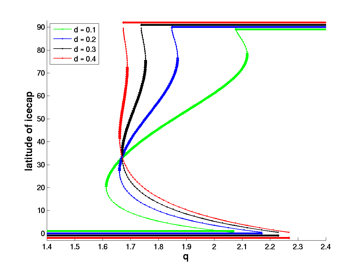
Latitude of ice margin as a function of a non-dimensional total solar irradiance in the diffusive energy balance climate model described by North 1975, for different values of the non-dimensional diffusion . Stable states are indicated by a thicker line.
When we were first starting out as graduate students, Max Suarez and I became interested in ice age theories and found it very helpful as a starting point to think about energy balance models for the latitudinal structure of the surface temperature. At about the same time, Jerry North had simplified this kind of model to its bare essence: linear diffusion on the sphere with constant diffusivity, outgoing infrared flux that is a linear function of surface temperature, and absorbed solar flux equal to a specified function of latitude multiplied by a co-albedo that is itself a function of temperature to capture the different planetary albedos for ice-free and ice-covered areas. Playing with this kind of “toy” model is valuable pedagogically — I certainly learned a lot by building and elaborating this kind of model — and can even lead to some nuggets of insight about the climate system.
The response of a 1km non-rotating doubly periodic model of radiative-convective equilibrium to an increase in surface temperature, in increments of 2K. Left: temperature, showing a moist-adiabatic response; Right: fraction of area with cloud at each height, showing an upward displacement of upper tropospheric clouds. From Kuang and Hartmann 2007.
The presence of cirrus clouds in the tropics warms the troposphere because infrared radiation is emitted to space from their relatively cold surfaces rather than the warmer temperatures below the clouds. The response of these clouds can be important as feedbacks to climate change. A reduction in the area covered by these high clouds would be a negative feedback to warming. [7/25/13: Several readers have pointed out that a reduction in the areas of high cloud cover would be a negative infrared feedback but a positive shortwave feedback and that the net effect could go either way.] An increase in the average height of these clouds with warming, resulting in a colder surface than would be the case if this height did not increase, would be a positive feedback. It is the latter that I want to discuss here. GCMs have shown a positive feedback due to increasing height of tropical cirrus since the inception of global modeling (e.g., Wetherald and Manabe, 1980). This is probably the most robust cloud feedback in GCMs over the years and is one reason that the total cloud feedbacks in GCMs tend to be positive. This increase in cloud top height has, in addition, a clear theoretical foundation, formulated as the FAT (Fixed Anvil Temperature) hypothesis by Hartmann and Larson, 2002.
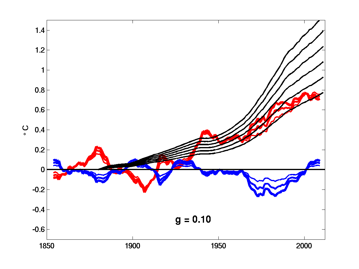
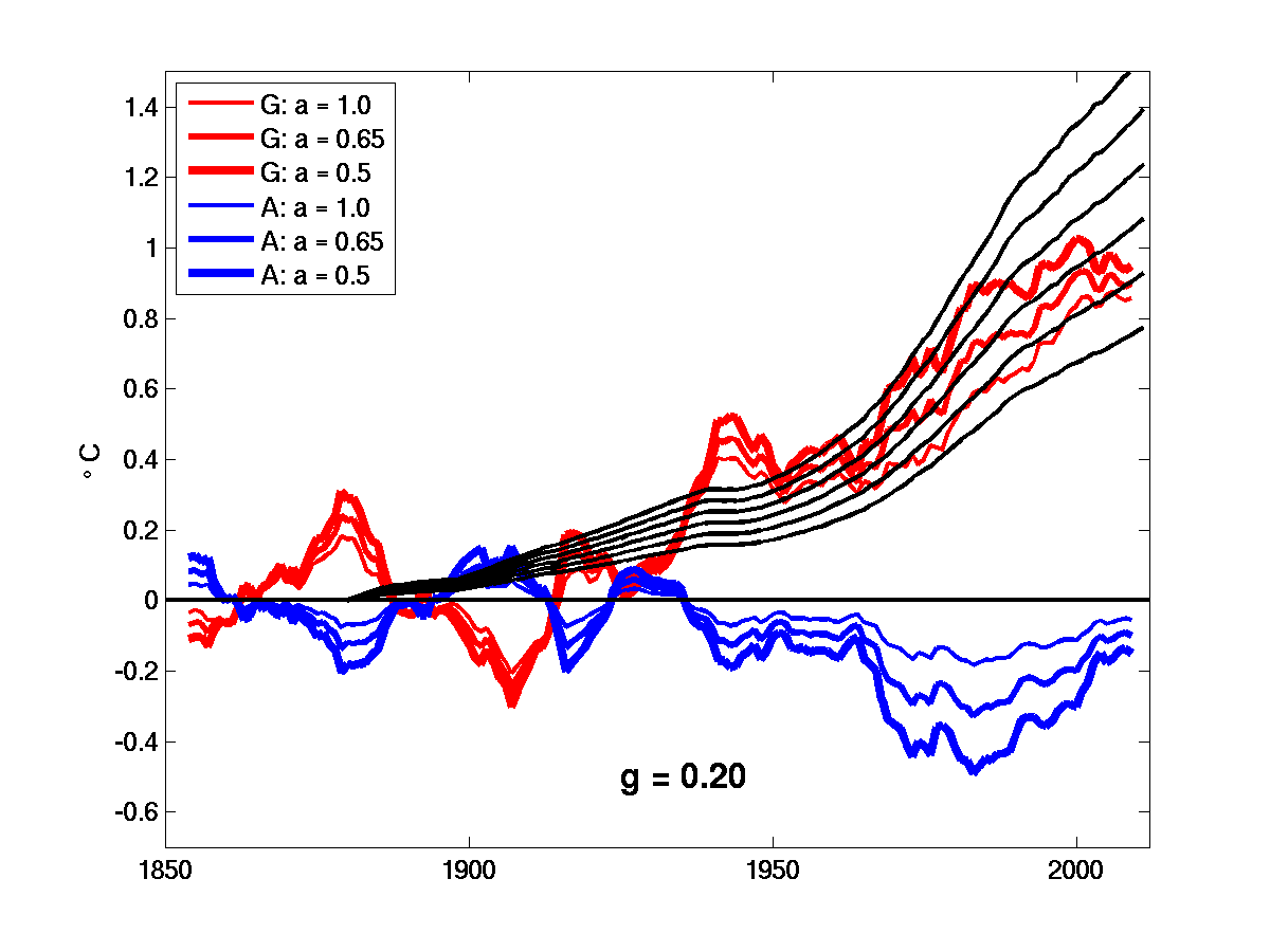
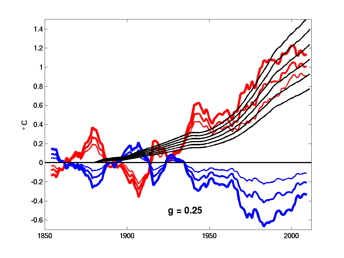
Rough estimates of the WMGG (well-mixed greenhouse gas — red) and non-WMGG (blue) components of the global mean temperature time series obtained from observed (HADCRUT4) Northern and Southern Hemisphere mean temperatures and different assumptions about the ratio of the Northern to Southern Hemisphere responses in these two components. Black lines are estimates of the response to WMGG forcing for 6 different values of the transient climate response TCR (1.0, 1.2, 1.4, 1.6, 1.8, 2.0C).
How can we use the spatial pattern of the surface temperature evolution to help determine how much of the warming over the past century was forced by increases in the well-mixed greenhouse gases (WMGGs: CO2, CH4, N2O, CFCs), assuming as little as possible about the non-WMGG forcing and internal variability. Here is a very simple approach using only two functions of time, the mean Northern and Southern Hemisphere temperatures. (See #7, #27, #35 for related posts.)
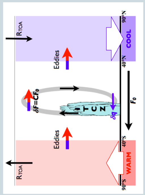
Schematic of the response of tropical rainfall to high latitude warming in one hemisphere and cooling in the other or, equivalently, to a cross-equatorial heat flux in the ocean. From Kang et al 2009.
When discussing the response of the distribution of precipitation around the world to increasing CO2 or other forcing agents, I think you can make the case for the following three basic ingredients:
the tendency for regions in which there is moisture convergence to get wetter and regions in which there is moisture divergence to get drier (“wet get wetter and dry get drier”) in response to warming (due to increases in water vapor in the lower troposphere — post #13);
the tendency for the subtropical dry zones and the mid-latitude storm tracks to move polewards with warming;
the tendency for the tropical rainbelts to move towards the hemisphere that warms more.
There are other important elements we could add to this set, especially if one focuses on particular regions — for example, changes in ENSO variability would affect rainfall in the tropics and over North America in important ways . But I think a subset of these three basic ingredients, in some combination, are important nearly everywhere. I want to focus here on 3) the effect on tropical rain belts of changing interhemispheric gradients.
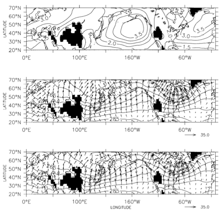
Lower panel: the observed (irrotational) component of the horizontal eddy sensible heat flux at 850mb in Northern Hemisphere in January along with the mean temperature field at this level. Middle panel: a diffusive approximation to that flux. Upper panel: the spatially varying kinematic diffusivity (in units of ) used to generate the middle panel. From Held (1999) based on Kushner and Held (1998).
Let’s consider the simplest atmospheric model with diffusive horizontal transport on a sphere:
.
Here is the energy input into the atmosphere as a function of latitude , is the outgoing infrared flux linearized about some reference temperature , is the heat capacity of a tropospheric column per unit horizontal area , and is a kinematic diffusivity with units of (length)2/time. Think of the energy input as independent of time and, for the moment, think of as just a constant.
(Left) Sea surface temperature averaged over the North Atlantic (75-7.5W, 0-60N), in the HADGEM2-ES model (ensemble mean red; standard deviation yellow) compared with observations (black), as discussed in Booth et al 2012. (Right) Upper ocean (< 700m) heat content in this model averaged over the same area, from Zhang et al 2013 ( green = simulation with no anthropogenic aerosol forcing, kindly provided by Ben Booth.)
A paper by Booth et al 2012 has attracted a lot of attention because of the claim it makes that the interdecadal variability in the North Atlantic is in large part the response to external forcing agents, aerosols in particular, rather than internal variability. This has implications for estimates of (transient) climate sensitivity but it also has very direct implications for our understanding of important climate variations such as the recent upward trend in Atlantic hurricane activity (linked to the recent rapid increase in N.Atlantic sea surface temperatures) and drought in the Sahel in the 1970’s (linked to the cool N. Atlantic in that decade). I am a co-author of a recent paper by Rong Zhang and others (Zhang et al 2013) in which we argue that the Booth et al paper and the model on which it is based do not make a compelling case for this claim.
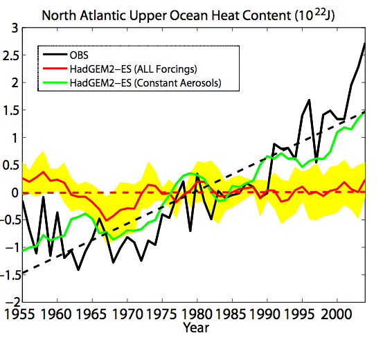
Anomalies in near surface air temperature over land (1979-2008) averaged over Asia and the months of June-July-August from CRUTEM4 (green) — and as simulated by atmosphere/land models in which oceanic boundary conditions are prescribed to follow observations (gray shading). See text and Post #32 for details.
This is a follow up to Post #32 on Northern Hemisphere land temperatures as simulated in models in which sea surface temperatures (SSTs) and sea ice extent are prescribed to follow observations. I am interested in whether we can use simulations of this “AMIP” type to learn something about how well a climate model is handling the response of land temperatures to different forcing agents such as aerosols and well-mixed greenhouse gases. If a model forced with prescribed SST/ice boundary conditions and prescribed variations in the forcing agents does a reasonably good job of simulating observations, we can then ask how much of this response is due to the SST variations and how much is due to the forcing agents (assuming linearity). If the response to SST variations is robust enough, we have a chance to subtract it off and see if different assumptions about aerosol forcing, in particular, improve or degrade the fit to observations.


 of longitude within the tropics (30S-30N) is shown. The ITCZ is located at
  in the upper panel and
  in the lower panel. Simulations described in
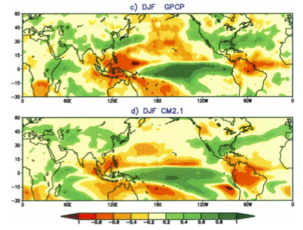
 in the diffusive energy balance climate model described by
  . Stable states are indicated by a thicker line.
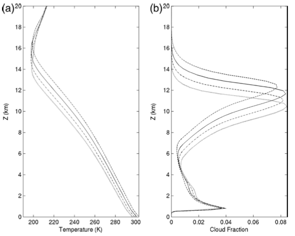
 ) used to generate the middle panel. From
  .
. is the energy input into the atmosphere as a function of latitude
  ,
,  is the outgoing infrared flux linearized about some reference temperature
  ,
,  is the heat capacity of a tropospheric column per unit horizontal area
  , and
, and  is a kinematic diffusivity with units of (length)2/time. Think of the energy input as independent of time and, for the moment, think of
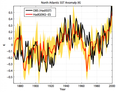
Recent Comments