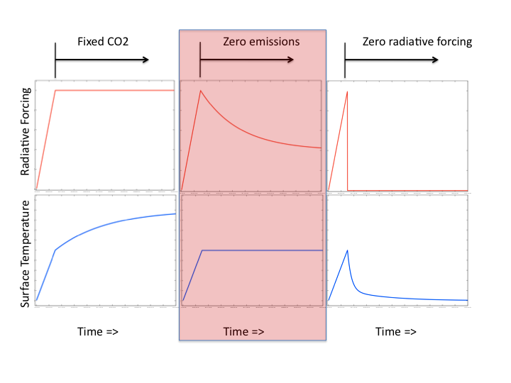
Schematic of three different idealized global warming scenarios. The time period is roughly 1,000 years and each scenario starts with the CO2 increase and warming from the anthropogenic pulse of emission in the 20th and 21st centuries. On the left, emissions are slowed so that CO2 is maintained at the level reached at the end of this pulse. In the center, emissions are eliminated at the end of the pulse, resulting in slow decay of CO2. On the right, CO2 levels are abruptly returned to pre-industrial levels —perfect geoengineering — a scenario useful for isolating the recalcitrant component of warming discussed in post #8.
If we stop emitting CO2 at some future time how would surface temperature evolve over the ensuing decades and centuries — ignoring all other forcing agents? This question (or closely related questions) has been looked at using a number of models of different kinds, including Allen et al, 2009, Matthews et al, 2009, Solomon et al, 2009, and Frolicher and Joos, 2010. These models agree on a simple qualitative result: global mean surface temperatures stay roughly level for as long as a millennium, at the value achieved at the time at which emissions are discontinued, as illustrated schematically in the middle panels above.
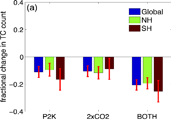
From Held and Zhao 2011, a simulation with an atmospheric model of the change in the number of tropical cyclones that form over each hemisphere and over the globe when sea surface temperatures (SSTs) are raised uniformly by 2C (labelled P2K), when the CO2 is doubled with fixed SSTs, and when SSTs and CO2 are increased together.
Suppose that we have a model of the climatic response to gradually increasing CO2, and we examine the globally-averaged incoming top-of-atmosphere flux, , as a function of time (using a large ensemble of runs of the model to average out internal variability). Letting refer to the difference between two climate states, for example the difference between the climates of 2100 and 2000 in a particular model, we end up looking at an expression like
where is the global mean surface temperature and refers to all of the other things on which depends. Here is the CO2 concentration, or, to the extend the useful range of this linearization, log(CO2). The forcing might be defined as . We typically go a step further and write so that we can think of this last term as a feedback, modifying the radiative restoring strength,
i.e, so that . While this is a formal manipulation that you can always perform if you want to, it is obviously more useful when is actually more or less proportional to . Ideally, there is a causal chain: => => . But what if the change in due to an increase in CO2 results from some other causal chain that doesn’t pass through the warming of the surface (or the warming of the strongly coupled surface-troposphere system)?
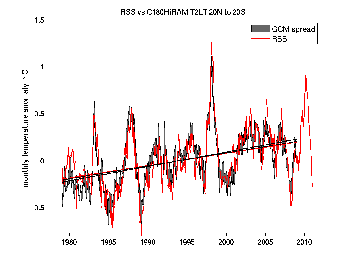
Lower tropospheric MSU monthly mean anomalies, averaged over 20S to 20N, as estimated by Remote Sensing Systems – RSS (red) and the corresponding result from three realizations of the GFDL HiRAMC180 model (black) using HadISST1 ocean temperatures and sea ice coverage. Linear trends also shown. (Details in the post.)
Motivated by the previous post and Fu et al 2011 I decided to look in a bit more detail at the vertical structure of the tropical temperature trends in a model that I have been studying and how they compare to the trends in the MSU/AMSU data. The model is an atmosphere/land model using as boundary condition the time-evolving sea surface temperatures and sea ice coverage from HadISST1. It is identical to the model that generates the tropical cyclones discussed in Post #2 (and the animation of outgoing infrared radiation in Post #1). It has the relatively high horizontal resolution, for global climate models, of about 50km. Three realizations of this model, starting with different initial conditions, for the period covering 1979-2008, have been provided to the CMIP5 database, and it is these three runs that I will use in this discussion. The model also has prescribed time-evolving well-mixed greenhouse gases, aerosols (including stratospheric volcanic aerosols), solar cycle, and ozone. The atmospheric and land states are otherwise predicted.
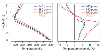
Results from a high resolution model of horizontally homogeneous radiative-convective equilibrium, Romps 2011. Left: equilibrium temperature profiles for 3 values of CO2 compared to an observed tropical profile. Right: the temperature differences compared to the response to doubling CO2 in an ensemble of CMIP3 global climate models.
As a moist parcel of air ascends it cools as it expands and does work against the rest of the atmosphere. If this were the only thing going on, the temperature of the parcel would decrease at 9.8K/km. But once the water vapor in the parcel reaches saturation some of this vapor condenses and releases its latent heat, compensating for some of the cooling (you get about 45K of warming from latent heat release when a typical parcel rises from the tropical surface to the upper troposphere). A warmer parcel contains more water vapor when it becomes saturated, so it condenses more vapor as it rises, and temperature decreases with height more slowly. That is, the moist adiabatic lapse rate, , decreases with warming.
To say something about the warming of the tropical atmosphere, rather than that of a moist adiabat, we need to argue that the tropical troposphere is close to a moist adiabat and remains close as it warms. The upper troposphere will then warm more than the lower troposphere. This is precisely what happens in our global climate models. The consistency or inconsistency of this prediction with observations, particularly the Microwave Sounding Unit (MSU) temperatures, is a long-standing and important issue A failure of the upper troposphere to warm as much as anticpated by this simple argument would signal a destabilization of the tropics — rising parcels would experience a larger density difference with their environment, creating more intense vertical accelerations — affecting all tropical phenomena involving deep convection. I like to refer to warming following the moist adiabat as the most “conservative” possible — having the least impact on tropical meteorology.
Animation of horizontally homogeneous non-rotating radiative-convective equilibrium courtesy of Caroline Muller. The model isSAM (System for Atmospheric Modeling) the principal architect of which is Marat Khairoutdinov. Transparent shading is condensate concentration; colors on the surface indicate near-surface air temperature. See text for further description.
The starting point for most of my thinking regarding climate sensitivity is the simple 1-dimensional radiative-convective model introduced by Suki Manabe and Dick Wetherald in 1967. See also Manabe and Strickler, 1964. For an early review of this kind of modeling, see Ramanathan and Coakley, 1978. Sadly, Dick Wetherald passed away very recently; although it is a very small gesture, I would like to dedicate this post to his memory.
A model configuration used to study how temperature variations in the equatorial Pacific force temperature variations in other ocean basins and the land. Figure courtesy of Gabriel Lau.
Consider a simple energy balance model for the oceanic mixed layer (+ land + atmosphere) with temperature and effective heat capacity . The net downward energy flux at the top-of-atmosphere is assumed to consist of a radiative relaxation, , plus some noise, . With imposed flux from the deep ocean to the mixed layer, :
The assumption is that there is no external radiative forcing due to volcanoes or increasing CO2, etc. Can we use a simple one-box model like this to connect observations of interannual variability in and to climate sensitivity?
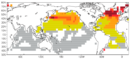
From DelSole et al, 2011 (pdf). The component of sea surface temperature variability that maximizes its integral time scale, obtained from the combination of 14 control runs of CMIP3 climate models.
This is a continuation of the previous post in which I analyze the sources of my confidence that the warming trend of the past half-century is dominated by external forcing.
Taking a long control integration of CM2.1, a GCM that I have talked about here before, I’ve used the last 2,000 years from the simulation described by Wittenberg, 2009, and located the period with the largest positive 50-year trend in global mean surface air temperature. The picture below is of the trend at each point, the global average of which is 0.41C. The average over the Northern Hemisphere only is about twice as large.
Suppose that most of the global mean surface warming in the past half century was due to internal variability rather than external forcing, contrary to one of the central conclusions in the IPCC/AR4/WG1 Summary for Policymakers. Let’s think about the implications for ocean heat uptake. Considering the past half century in this context is convenient because we have direct, albeit imprecise, estimates of ocean heat uptake over this period.
Set the temperature change in question, , equal to the sum of a forced part and an internal variability part: , with , so is the fraction of the temperature change that is forced. The assumption is that this is a linear superposition of two independent pieces, so I’ll write the heat uptake as .
When the surface of the Earth warms due to external forcing, we expect the Earth to take up heat. But what do we expect when the surface warms due to internal variability? Can we use observations of heat uptake to constrain ?
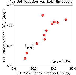
From Son et al 2010, based on the CCMVal ensemble of models, the decorrelation time of the Southern annular mode (SAM) plotted against the simulated latitude of the surface westerlies. Also included is an estimate from NCEP-NCAR reanalysis.
A series of studies over the past decade, starting with Thompson and Solomon 2002, have built a very strong case that the ozone hole in the Southern Hemisphere (SH) stratosphere has caused a poleward shift in the SH surface westerlies and associated eddy fields, especially during the southern summer. The poleward shift is often described as a trend towards a more positive phase of the Southern Annular Mode (SAM). The SAM is a mode of atmospheric internal variability characterized by north-south shifts in the surface westerlies.
The mechanism by which the ozone hole causes this poleward shift is a hot topic in dynamical meteorology. Not only is this response to the ozone hole important in itself, but related mechanisms likely govern the effects on the troposphere of stratospheric perturbations due to volcanic eruptions, the solar cycle, and internal variability. The starting point is the cooling of the lower stratosphere in the vicinity of the ozone hole, due to loss of UV absorption, thereby changing the north-south temperature gradient and associated wind fields in the lower stratosphere. But there are a lot of competing ideas about how altered lower stratospheric winds and temperatures in turn affect the fluxes of angular momentum that maintain the surface westerlies. (Some of my own lectures on the basic dynamics controlling the surface westerlies, including the key role of transport of angular momentum associated with the midlatitude storm tracks, can be found here.) GCMs consistently simulate a poleward shift in response to the ozone hole but of varying magnitude. They also consistently simulate a poleward shift due to increasing CO2.
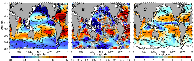
From Durack and Wijffels, 2010: A) Climatological surface salinity (0.5 pss contour), averaged over 1950-2000; B) the linear trend over these 50 years (pss/50 years) ; and C) the NOCS Southampton estimate of net climatological freshwater flux from ocean to atmosphere (m/yr).
In post #13, I discussed the argument that warmer temperatures => more water vapor in the atmosphere => more transport of water away from regions from which the atmosphere habitually extracts water, and more transport to regions into which the atmosphere habitually adds water. The consequence is the expectation that “the wet get wetter and the dry get drier” if by wet/dry we mean regions with precipitation (P) greater than/less than evaporation (E). In that post, I effectively ignored the presence of land. Land introduces a variety of complications that make this kind of argument more difficult, most obviously because of the constraint that P must be greater than E on the time scales of interest (ie. changes in water storage on land can be ignored and runoff must be positive). I am going to continue to ignore the existence of land (and glaciers) in this post!
What is the evidence for trends in P or E or P-E over the oceans? Trends in the ocean salinity field promise to provide a test of our understanding — it is also helpful that the oceans provide a low-pass filter to noisy precipitation signals.


 , as a function of time (using a large ensemble of runs of the model to average out internal variability). Letting
  refer to the difference between two climate states, for example the difference between the climates of 2100 and 2000 in a particular model, we end up looking at an expression like
 refers to all of the other things on which
  is the CO2 concentration, or, to the extend the useful range of this linearization, log(CO2). The forcing
  might be defined as
  . We typically go a step further and write
  so that we can think of this last term as a feedback, modifying the radiative restoring strength,
 . While this is a formal manipulation that you can always perform if you want to, it is obviously more useful when
  is actually more or less proportional to
  . Ideally, there is a causal chain:
  =>
=> 
 Results from a high resolution model of horizontally homogeneous radiative-convective equilibrium,
  , decreases with warming.
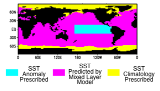 A model configuration used to study how temperature variations in the equatorial Pacific force temperature variations in other ocean basins and the land. Figure courtesy of Gabriel Lau.
 . The net downward energy flux at the top-of-atmosphere
  is assumed to consist of a radiative relaxation,
  , plus some noise,
  :
:
 , with
  , so
, so  is the fraction of the temperature change that is forced. The assumption is that this is a linear superposition of two independent pieces, so I’ll write the heat uptake as
  .
.
Recent Comments