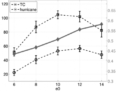
Globally integrated, annual mean tropical cyclone (TC) and hurricane frequency simulated in the global model described in Post #2, as a function of a parameter in the model’s sub-grid moist convection closure scheme, from Zhao etal 2012.
It is difficult to convey to non-specialists the degree to which climate models are based on firm physical theory on the one hand, or tuned (I actually prefer optimized) to fit observations on the other. Rather than try to provide a general overview, it is easier to provide examples. Here is one related to post #2 in which I described the simulation of hurricanes in an atmospheric model.
Anomalies in annual mean near surface air temperature over land (1979-2008), averaged over the Northern Hemisphere, from CRUTEM4 (green) and as simulated by an ensemble of atmosphere/land models in which oceanic boundary conditions are prescribed to follow observations.
As discussed in previous posts, it is interesting to take the atmosphere and land surface components of a climate model and run it over sea surface temperatures (SSTs) and sea ice extents that, in turn, are prescribed to evolve according to observations. In Post #2 I discussed simulations of trend and variability in hurricane frequency in such a model, and Post #21 focused on the vertical structure of temperature trends in the tropical troposphere. A basic feature worth looking at in this kind of model is simply the land temperature – or, more precisely, the near-surface air temperature over land. How well do models simulate temperature variations and trends over land when SSTs and ice are specified? These simulations are referred to as AMIP simulations, and there are quite a few of these in the CMIP5 archive, covering the period 1979-2008.
Relative humidity evolution over one year in a 50km resolution atmospheric model
in the upper (250hPa) and lower (850hPa) troposphere.
In their 1-D radiative-convective paper of 1967, Manabe and Wetherald examined the consequences for climate sensitivity of the assumption that the tropospheric relative humidity (RH) remains fixed as the climate is warmed by increasing CO2. In the first (albeit rather idealized) GCM simulation of the response of climate to an increase in CO2, the same authors found, in 1975, that water vapor did increase throughout the model troposphere at roughly the rate needed to maintain fixed RH. The robustness of this result in the world’s climate models in the intervening decades has been impressive to those of us working with these models, given the differences in model resolution and the underlying algorithms, a robustness in sharp contrast to the diversity of cloud feedbacks in these same models.
Percentage change in the precipitation falling on days within which the daily precipitation is above the pth percentile (p is horizontal axis) as a function of latitude and averaged over longtitude, over the 21st century in a GCM projection for a business-as-usual scenario, from Pall et al 2007.
(I have added a paragraph under element (1) below in response to some off-line comments — Aug 15)
When I think about global warming enhancing “extremes”, I tend to distinguish in my own mind between different aspects of the problem as follows (there is nothing new here, but these distinctions are not always made very explicit):
1) increases in the frequency of extreme high temperatures that result from an increase in the mean of the temperature distribution without change in the shape of the distribution or in temporal correlations
The assumption that the distribution about the mean and correlations in time do not change certainly seems like an appropriately conservative starting point. But if you look far out on the distribution, the effects on the frequency of occurrence of days above a fixed high temperature, or of consecutive occurrences of very hot days (heat waves), can be surprisingly large. Just assuming a normal distribution, or playing with the shape of the tails of the distribution, and asking simple questions of this sort can be illuminating. I’m often struck by the statement that “we don’t care about the mean; we care about extremes” when these two things are so closely related (in the case of temperature). Uncertainty in the temperature response translates directly into uncertainty in changes in extreme temperatures in this fixed distribution limit. It would be nice if, in model projections, it was more commonplace to divide up the responses in extreme temperatures into a part due just to the increase in mean and a part due to everything else. It would make it easier to see if there was much that was robust across models in the “everything else” part. And it also emphasizes the importance of comparing the shape of the tails of the distributions in models and observations. Of course from this fixed-distribution perspective every statement about the increase in hot extremes is balanced by one about decreases in cold extremes.
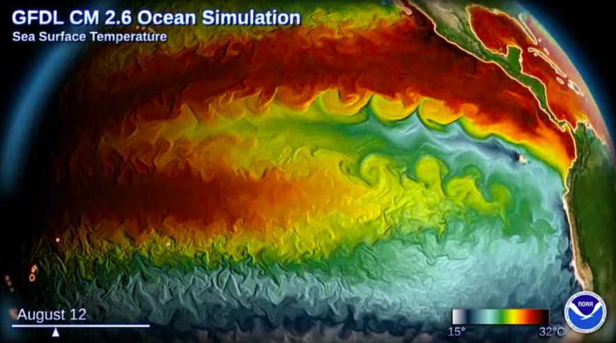
Animation of the sea surface temperature in a coupled climate model under development at GFDL,
the ocean component having an average resolution of roughly 0.1 degree latitude and longitude.
Click HERE for the animation. (Visualization created by Remik Ziemlinski; model developed by T. Delworth, A. Rosati, K. Dixon, W. Anderson using MOM4 as the oceanic code base.)
As models gradually move to finer spatial resolution we naturally expect to gradually improve our simulations of atmospheric and oceanic flows. But things get especially interesting when one passes thresholds at which new phenomena are simulated that were not present in anything like a realistic form at lower resolution. The animation illustrates what happens after one passes through an important oceanic threshold, allowing mesoscale eddies to form, filling the oceanic interior with what we refer to as geostrophic turbulence. At resolutions too coarse to simulate the formation of these eddies, flows in ocean models tend to be quite laminar except for some relatively large scale instabilities of intense currents of the kind seen in the snapshot north of the equator in the Eastern Pacific. (For a transition comparably fundamental in atmospheric models, one has to turn to the point at which global models begin to resolve the deep convective elements in the tropical atmosphere — see for example Post #19).
Animations of the near surface temperature (top) and upper tropospheric zonal winds (bottom) in an idealized dry atmospheric model. The first 500 days of spinup from a state of rest are shown at one frame per day for the entire globe.
As a change of pace from discussions of climate sensitivity, I’ll describe an idealized atmospheric model that I think of as an important element in a model hierarchy essential to our thinking about atmospheric circulation and climate.
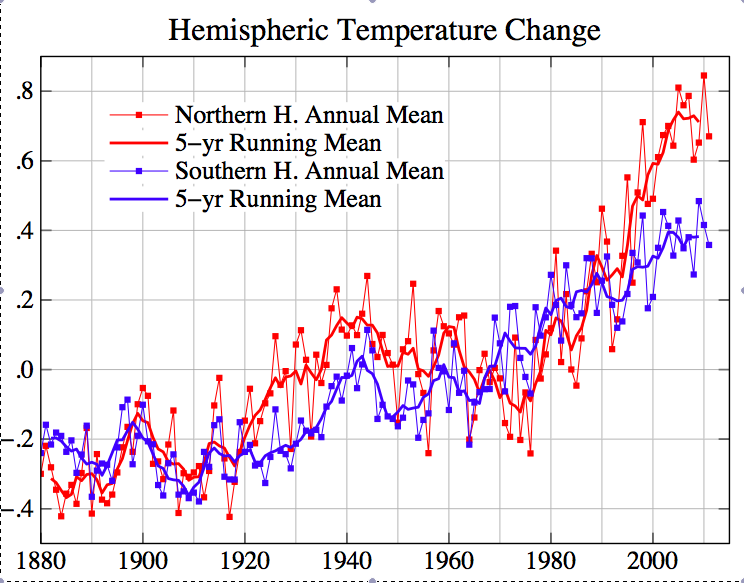
GISTEMP annual mean surface temperatures (degrees C)
for the Northern and Southern Hemispheres.
Here’s an argument that suggests to me that the transient climate response (TCR) is unlikely to be larger than about 1.8C. This is roughly the median of the TCR’s from the CMIP3 model archive, implying that this ensemble of models is, on average, overestimating TCR
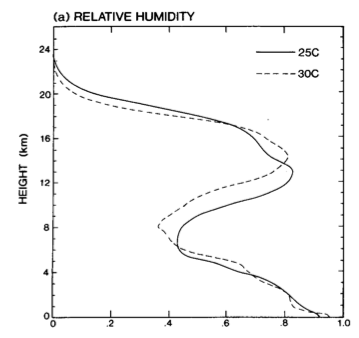
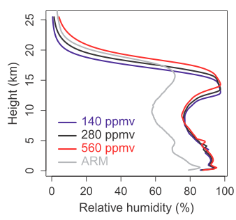
Time and spatially averaged relative humidity profiles from radiative-convective equilibrium simulations with cloud-resolving models. The figure on the left is from Held et al, 1993 and shows results from two simulations differing by 5C in the prescribed surface temperature. That on the right is from Romps 2011 and shows the result of changing the CO2 and adjusting surface temperatures to keep the net flux at the top of the atmosphere unchanged. (Also shown on the right is the observed profile at a tropical western Pacific ARM site.)
Regarding water vapor or, equivalently, relative humidity feedback, we can think of theory/modeling as providing a “prior” which is then modified by observations (trends, interannual variability, Pinatubo response). My personal “prior” is that relative humidity feedback is weak. or, conversely, that the strength of water vapor feedback in our global models is about right.
In justifying this prior, I like to start with the rather trivial argument, already mentioned in the last post, that the amount of water vapor in the atmosphere cannot possibly stay unchanged as the climate cools since many regions will become supersaturated, including the upper tropical troposphere where most of the water vapor feedback is generated.. So to expect specific humidity to remain unchanged as the climate warms requires the present climate to be close to a distinguished point as a function of temperature – the point at which water vapor stops increasing as temperatures increase. Its not impossible that we do reside at such a point, but you’re going to have work pretty hard to convince me of that — it doesn’t strike me as a plausible starting point.
Of course, there is also the community’s collective experience with global atmospheric models over the past several decades. Less familiarly, there is experience more recently with the kind of “cloud-resolving” models (CRMs) discussed in Posts #19-20. I am going to focus on the latter here. This will have the advantage of introducing what I consider to be the physical mechanism that could most plausibly alter the strength of water vapor feedback.
Some feedbacks in AR4 models, from Held and Shell 2012. The three red columns on the right provide the traditional perspective: the “Planck feedback”– the response to uniform warming of surface and troposphere with fixed specific humidity (), the lapse rate feedback at fixed specific humidity (), and the water vapor feedback (). The three blue columns on the left provide an alternative perspective — with the fixed relative humidity uniform warming feedback (), the fixed relative humidity lapse rate feedback, (), and the relative humidity feedback (). The sum of the three terms, shown in the middle black column, is the same from either perspective. Surface albedo and cloud feedbacks are omitted. Each model is a dot.
This is the continuation of the previous post, describing how we can try to simplify the analysis of climate feedbacks by taking advantage of the arbitrariness in the definition of our reference point, or equivalently, in the choice of variables that we use to describe the climate response. There is nothing fundamentally new here — it is just making explicit the way that many people in the field actually think, myself included. And if you don’t like this reformulation, that’s fine — it’s just an alternative language that you’re free to adopt or reject.
This post is concerned with arbitrariness in the terminology we use when discussing climate feedbacks. The choice of terminology has no affect on the underlying physics, but it can, I think, affect the picture we keep in our minds as to what is going on, and can potentially affect the confidence we have in this picture.
In feedback analyses of a climate response to some radiative forcing, we start with a reference response, the response “in the absence of feedbacks”, and then we look at how this reference response is modified by feedbacks. An electrical circuit analogy often comes to mind, with the reference response analogous to the unambiguous input into a circuit. But the choice of reference response in our problem is ultimately arbitrary. The following is closely based on the introductory section of Held and Shell 2012.


 Globally integrated, annual mean tropical cyclone (TC) and hurricane frequency simulated in the global model described in Post #2, as a function of a parameter in the model’s sub-grid moist convection closure scheme, from Zhao etal 2012.
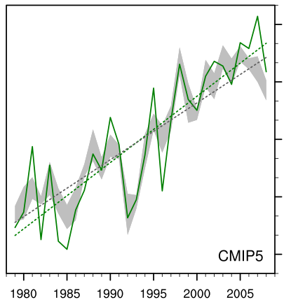
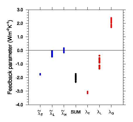
 ), the lapse rate feedback at fixed specific humidity (
 ), and the water vapor feedback (
 ). The three blue columns on the left provide an alternative perspective — with the fixed relative humidity uniform warming feedback (
 ), the fixed relative humidity lapse rate feedback, (
 ), and the relative humidity feedback (
 ). The sum of the three terms, shown in the middle black column, is the same from either perspective. Surface albedo and cloud feedbacks are omitted. Each model is a dot.
Recent Comments